Corpus
Slides: Integration
The lab's transcriptions of the decks embedded on https://www.iit.wiki/axioms-and-postulates/integration: each slide's text as the deck shows it, and in square brackets a description of each diagram, which is the transcriber's and not the deck's.
Slideshow 1: Integration Postulate - 08/2023
Source page: Integration Source deck: Integration Postulate (37 slides)
Title slide (slide 1)
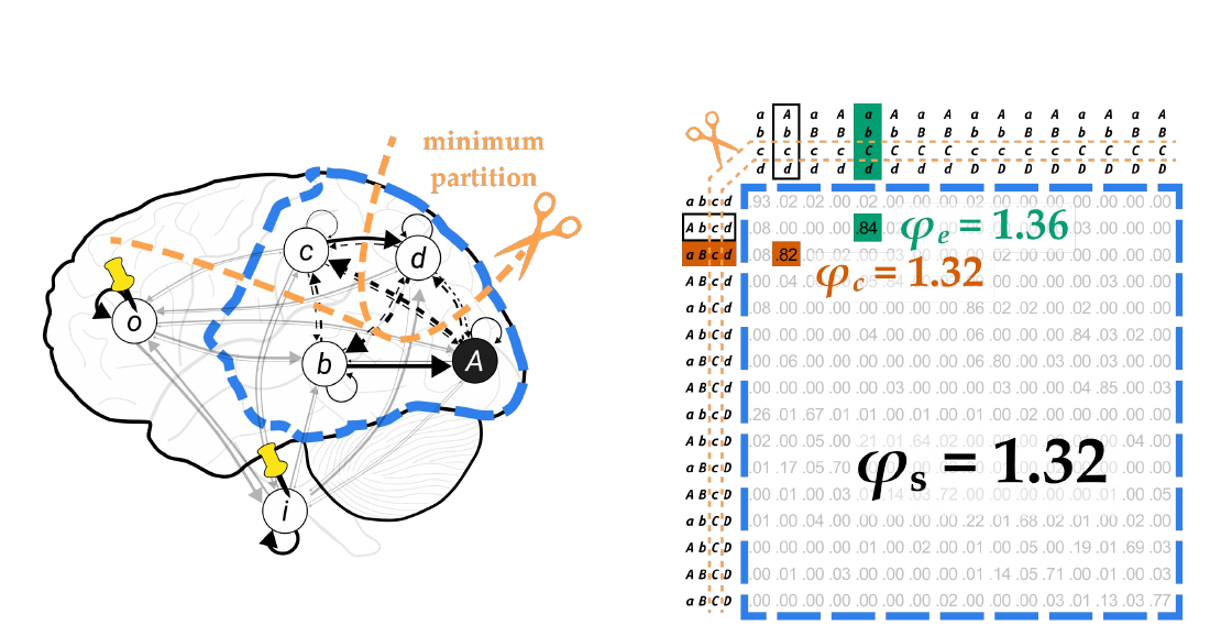
[On the left is the brain with the six units. A dashed blue line encloses the candidate system A, B, C and D, shown in its current state (A ON, the others OFF), and units O and I carry yellow pushpins. Dashed orange lines labelled "minimum partition," with an orange pair of scissors, cut across the candidate, separating A and B from C and from D; several arrows between the parts are dashed to show that they are cut. On the right is the TPM of the candidate system, with the current state boxed in black, the cause state marked in orange and the effect state in green, and dashed orange lines and a pair of scissors marking the partition across its column headings. Large lettering over the table reads φe = 1.36 in green, φc = 1.32 in orange, and, largest, φs = 1.32 in black. A red "(click)" prompt invites the reader to advance.]
From axiom to postulate (slides 2–5)
Axiom: Experience is unitary: it is a whole, irreducible to separate experiences.
How can we formulate this phenomenal property in physical terms—that is, in terms of cause–effect power?
Postulate: The cause–effect power of the substrate of consciousness must be unitary: it must specify its cause–effect state as a whole set of units, irreducible to separate subsets of units.
Note that these slides give a conceptual overview of the postulate without going into the mathematics. Use the links to learn more about key concepts, and visit the Computing Φ page for technical details.

[Beneath the axiom is the round photograph of the wiki's sample experience, a first-person view of lying on a bed with a book in a bright room with wide windows. Below it, the lower part of the scene is shown split into two separate halves, each in its own circle with a dashed grey border, standing for separate experiences to which the whole cannot be reduced. A blue arrow leads from the axiom to the postulate, which is set above the question.]
Recap of the information postulate (slides 6–7)
Recall from the information postulate that we aimed to capture the specific cause–effect power of the candidate system in its current state (Abcd).
We did this by calculating the intrinsic information on the cause side and the effect side, which gave us the cause–effect state (aBcd–abCd).
[These slides repeat the figures of the Information deck: the candidate system ABCD on the substrate graph with O and I pinned, "current state Abcd" leading to the cause–effect state aBcd–abCd, and its TPM with the maximal intrinsic information iic* = 2.76 and iie* = 2.95.]
Specifying the cause–effect state as a whole (slides 8–9)
The integration postulate now requires that the current state specify its cause–effect state as a whole set of units.
Another way to say this is that the cause–effect power of Abcd must be irreducible: its cause–effect power cannot be reduced to, say, that of Ab and cd separately.
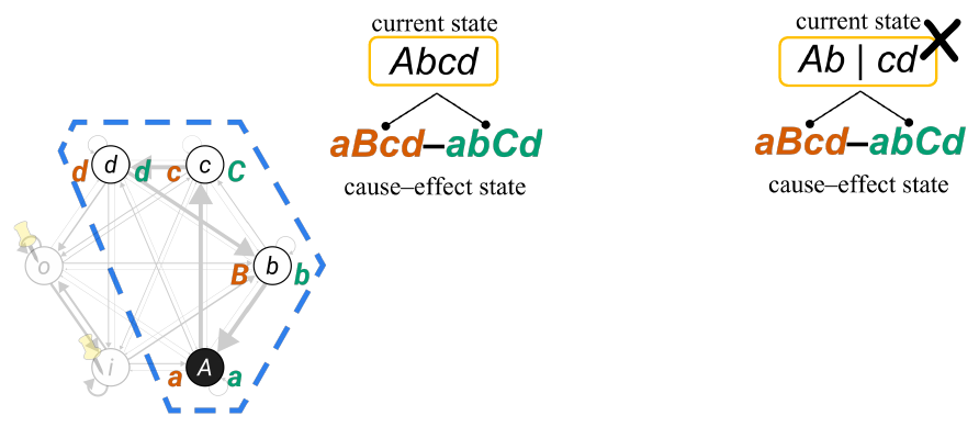
[On the left is the substrate graph with each candidate unit's cause and effect states written beside it in orange and green. In the middle, "current state Abcd," outlined in yellow, leads to the cause–effect state aBcd–abCd. On the right, the same diagram is drawn with the current state split as "Ab | cd," and a large black X marks it as not how the cause–effect state is specified.]
Partitioning the system (slides 10–14)
We assess integration using partitioning operations.
Note that for graphical simplicity, the substrate model will only show the current state and not the cause–effect state; but consider it there implicitly.
For example, on the substrate model, we see a partition of Abcd into the parts Ab, c, and d…
…which we can also illustrate roughly on the TPM.
Like in the information postulate slides, we're only showing the effect TPM here for graphical simplicity. But the complete partitioning operations are done on the cause TPM and effect TPM independently.
Technical details are in Computing Φ: Step 4—integration.
[On the substrate graph, dashed orange lines and an orange pair of scissors divide the candidate into three parts: A and B, C, and D. The same dashed orange lines, with a pair of scissors, run across the column headings of the TPM. In the text, the word "partition" is printed in orange. The graph and TPM appear with the φ values in the image for slide 36 below.]
Cuts (slides 15–17)
A partition comprises a set of unidirectional "cuts," as illustrated by the dashed connection arrows below.
In this case, the partition comprises nearly all possible cuts among parts Ab, c, and d; only the causal connection from part c to d is left intact.
Also note that connections within parts are left intact—this includes self-loops and, e.g., the connections between b and A.
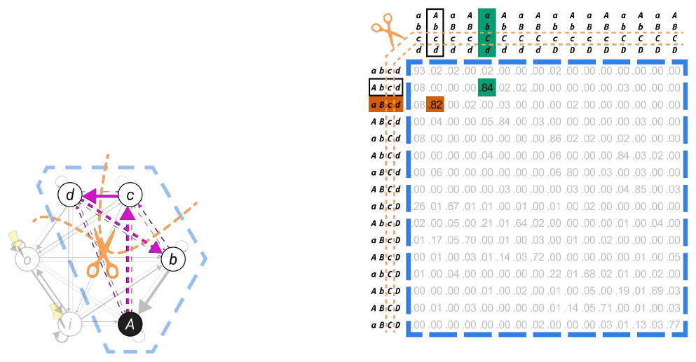
[On the partitioned substrate graph, every connection between the parts is highlighted in magenta. All of them are drawn as dashed lines, meaning they are cut (among them the thick arrow from A up to C and the arrow from D to B), except the arrow from C to D, which stays solid because it is left intact. Beside the graph, the TPM shows the same partition across its column headings.]
Cuts from the perspective of each part (slides 18–20)
It may be easier to see this by depicting the connections among parts, rather than individual units, as shown on the right.
A cut is thought about from the perspective of one part at a time, and a valid cut must sever all connections to or from that part (or both). Here, for example, the cut severs all connections to c.
A valid partition comprises cuts made to each of the parts. So, here, we have also cut all connections from d and all connections to and from Ab. All these cuts together make up the partition.
For details, see FAQ: What is a valid partition?
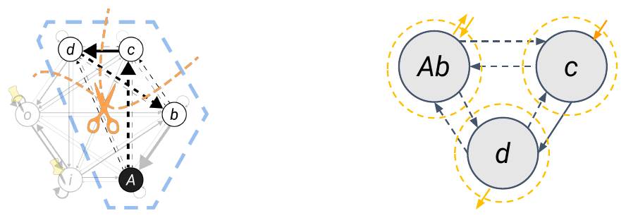
[To the right of the partitioned substrate graph is a simpler graph of the three parts, drawn as large grey circles labelled Ab, c and d, with arrows between them: dashed where a connection is cut, solid where it is intact (from c to d). On slide 19, a dashed yellow circle surrounds c, with a small yellow mark on its incoming side, showing that the cut severs all connections to c. On slide 20, every part has such a circle: Ab is marked on both sides (all connections to and from it cut), c on its incoming side, and d on its outgoing side. In the text, the word "cut" is printed in yellow.]
Comparing the partitioned and intact system (slides 21–26)
For a given partition, we are then able to calculate the integrated (intrinsic) information of the system (φs). The details for calculating φs can be found here.
The basic principle, however, is simple: We compare the intrinsic, specific cause–effect power of the partitioned system (left) with that of the intact system (right).
We can think of this as checking how the two versions of the system compare in specifying their cause–effect state.
Note that this is a rough, intuitive way of thinking about it; the math does not explicitly do it this way.
If the partitioned system specifies the cause–effect state as well as (or better than) the intact system, then φs is zero, and we can say that the system does not specify its cause–effect state as a whole.
Another way to say this is that such a system is reducible—its cause–effect power is not integrated or unitary.
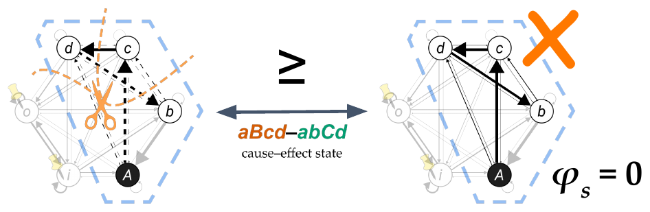
[The partitioned substrate graph (left) and the intact substrate graph (right) are joined by a double-headed arrow labelled with the cause–effect state aBcd–abCd. Between them stands a large "≥" sign, meaning that the partitioned system specifies the cause–effect state as well as or better than the intact one. Beside the intact graph is "φs = 0," and on slide 26 a large orange X is set over it. On slides 21 and 22, "φs = ?" is written over the TPM; on slides 23 and 24, a question mark stands between the two graphs.]
When φs is positive (slides 27–28)
But if the partitioned system specifies the cause–effect state less strongly than the intact system, then φs is positive and the system may be irreducible.
Another way to say this is that the cause–effect power of the system may be integrated or unitary.
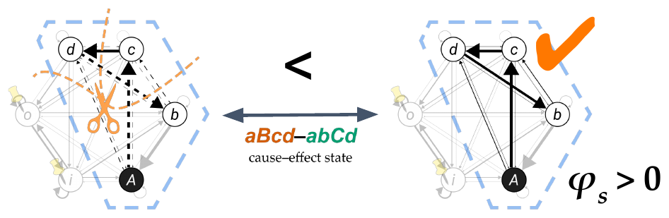
[The same pair of graphs, now with a large "<" sign between them, meaning that the partitioned system specifies the cause–effect state less strongly than the intact one. Beside the intact graph is "φs > 0," and on slide 28 a large orange check mark is set over it.]
The minimum partition (slides 29–33)
Why do we say the system "may be" irreducible if a partition yields a positive φs value?
Because we have to assess the φs of every possible partition. By the principle of minimal existence, we aim to discover the minimal partition—the one with the lowest normalized φs value.
In this case, the partition depicted is indeed the minimal partition, so we can conclude that Abcd is irreducible and thus fulfills the integration postulate.
Why do we use the minimum partition?
As an analogy, if we want to determine the degree to which this rope exists as "a rope," it wouldn't suffice to assess its strength in one of the strong sections.
We would rather have to check its strength in the most heavily frayed section: it can only exist as a unitary rope as much as this section allows.
Rope Image: Cartoon Vectors by Vecteezy
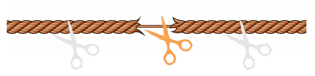
[A long brown twisted rope runs across the slide. Near its middle, a section is frayed down to a few thin strands. A bright orange pair of scissors is placed at the frayed section, and two faded grey pairs of scissors sit at strong sections to either side. On slide 32 the scissors are placed only at the strong sections.]
Minimal existence on the cause and effect sides (slides 34–36)
The principle of minimal existence is also applied in a second sense.
For a given partition, we calculate φ on the cause side and the effect side, and then take the minimum as the system integrated information (φs). This is because existence requires both cause and effect power; hence a substrate cannot exist as one substrate more than the least it is integrated on the cause or effect side.
For this system, the minimum partition is the one indicated, and therefore φs is 1.32—the value of φc. For technical details, see Computing Φ: Step 4—integration.
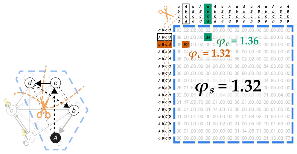
[The partitioned substrate graph sits beside the TPM, which shows the partition across its column headings, the current state boxed, the cause state in orange and the effect state in green. Over the table, large lettering reads φe = 1.36 in green and φc = 1.32 in orange, and below them, largest, φs = 1.32 in black. In the text, "cause side" is printed in orange and "effect side" in green.]
Summary slide (slide 37)
[The closing slide, labelled "summary," pairs the axiom and postulate from slide 5, with the photograph of the whole and its separate halves, with the diagram from slide 1: the brain with the minimum partition and the TPM with φe = 1.36, φc = 1.32 and φs = 1.32.]