Corpus
Slides: Foundations of IIT: Phenomenal & Physical Existence
The lab's transcriptions of the decks embedded on https://www.iit.wiki/foundations: each slide's text as the deck shows it, and in square brackets a description of each diagram, which is the transcriber's and not the deck's.
Slideshow 1: Existence - 0th Postulate - Dec. 2022
Source page: Foundations of IIT: Phenomenal & Physical Existence, section "0th Postulate" Source deck: Existence - 0th Postulate (37 slides)
Title slide (slide 1)
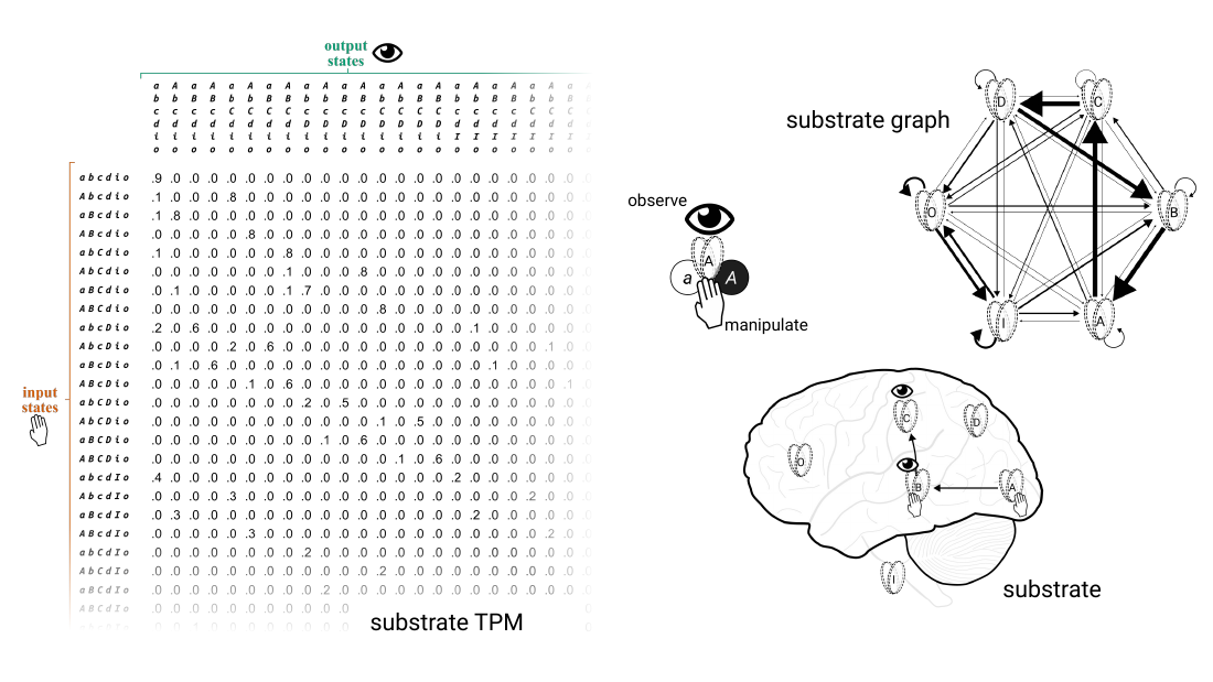
[The opening slide gathers the four elements the deck will introduce. On the left is a large substrate TPM, labelled "substrate TPM", whose rows are marked "input states" with a hand icon and whose columns are marked "output states" with an eye icon; each row and column is labelled with a state of the six units (for example, abcdio or AbCdIo). In the centre is a single unit shown in two states, OFF (a, white) and ON (A, black), with an eye labelled "observe" above it and a hand labelled "manipulate" below it. At top right is a substrate graph: six units (A, B, C, D, I, O) arranged in a hexagon, every unit connected to every other by arrows of varying thickness, each unit with a self-loop. At bottom right is an outline of the brain labelled "substrate", with the six units placed on it and arrows between some of them. A red "(click)" prompt invites the reader to advance.]
Manipulating and observing units (slides 2–5)
To assess the human brain as a substrate of consciousness, we must manipulate its constituent units and observe the effects of those manipulations.
The units we manipulate and observe could be neurons, but they could also be minicolumns, whole brain areas, or even molecules.
For example, here we've isolated six candidate units (A, B, C, D, I, O). We can manipulate any unit by changing its state, and we can observe the effect of this manipulation.
The units have two possible states, ON (uppercase) or OFF (lowercase).
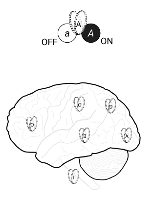
[An outline of the brain shows the six units scattered across it, each drawn as a small neuron-like icon bearing its letter. Beside it, a single unit is shown twice: white with a lowercase letter, labelled OFF, and black with an uppercase letter, labelled ON.]
Taking and making a difference (slides 6–9)
Let's say we manipulate D—for example, by stimulating it with an electric current—and we then observe D to be ON. If we do this many times with the same result, we may infer that D can "take a difference."
When we stimulate D, however, we might then also reliably observe unit O to be ON. This lets us infer that D can also "make a difference," in that its state appears to have an effect on the state of O (which, too, can "take a difference").
It's possible that we have observed mere correlations but not causation. But it's more reasonable to infer that D can indeed take and make difference—that it has cause–effect power.
We can also infer that this cause–effect power persists, also when we don't observe and manipulate. This reliable and persistent cause–effect power is shown graphically by arrows.
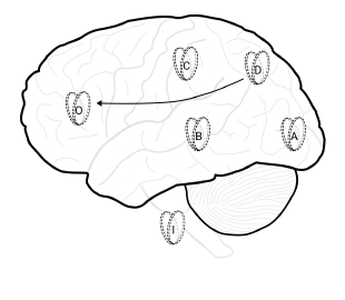
[In the earlier slides of this sequence, a hand labelled "Manipulate" acts on unit D and an eye labelled "Observe" watches unit O. On the last slide, shown here, an arrow runs from D to O across the brain, standing for D's reliable and persistent effect on O.]
Manipulation as setting a unit OFF (slides 10–13)
Note that a "manipulation" might also mean setting a unit to OFF.
For example, we might inject a negative current into A to keep it OFF, and observe that this reliably has the effect of turning unit O ON.
It's intuitive to describe these manipulations and observations as some sort of "causal interaction," but what does this mean? In IIT, cause–effect power is understood in strictly probabilistic, counterfactual terms:
The probability of unit O being ON is reliably higher than chance when unit A was OFF. Implicitly, therefore, if unit A had not been OFF, unit O would have had lower probability of being ON.
Such probabilities form the basis for quantifying the "raw" cause–effect power of a system—known as informativeness in the mathematical formalism of IIT.
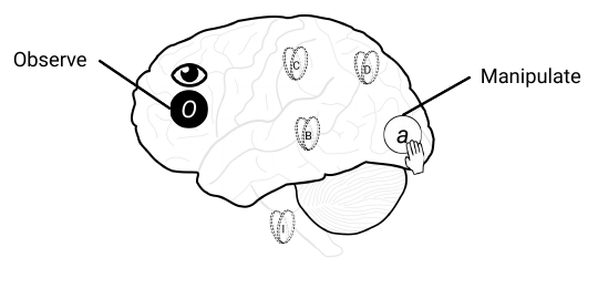
[On the brain outline, a hand labelled "Manipulate" holds unit A in its OFF state (white, lowercase a), while an eye labelled "Observe" watches unit O, shown ON (black, uppercase O).]
Summary of the postulate; tools to analyze cause–effect power (slides 14–15)
Tools to analyze cause–effect power: TPMs & substrate graphs
In sum, the existence postulate (or "0th" postulate) is simply the requirement that all the units we are assessing have cause–effect power. But to analyse cause–effect power in detail, two methodological tools will be helpful: TPMs and substrate graphs.
The transition probability matrix (slides 16–24)
A transition probability matrix (TPM) can help us quantify how some units (e.g., unit D) causally constrain some other units (e.g., unit O).
In the TPM, this is done by showing the probability of an output state (e.g., O OFF) given a specific input state (e.g., D ON).
To obtain the TPM of an input–output pair, we repeatedly set the inputs into all possible states, record the following states of the output, and compute the conditional probabilities of the output states.
Here is a cartoon representation of the experiment needed to obtain the TPM for input D to output O.
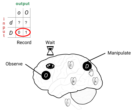
[The TPM is drawn as a small two-by-two table. Its rows are the input states of D (d = OFF, D = ON), marked "input" in red; its columns are the output states of O (o = OFF, O = ON), marked "output" in green. On the brain, a hand labelled "Manipulate" sets D to ON, an hourglass labelled "Wait" marks the passage of one time step, and an eye labelled "Observe" finds O ON. The result is entered in the table (labelled "Record"): the D row, circled in red, reads 0 under o and 1 under O, while the d row still holds question marks.]
Then repeat for another state of D—manipulating it, for example, to OFF.
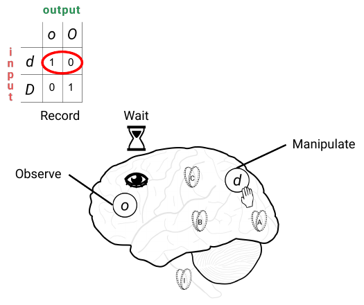
[Now the hand sets D to OFF (white, lowercase d), and after the wait the eye finds O OFF (white, lowercase o). The d row, circled in red, reads 1 under o and 0 under O; the D row keeps its earlier 0 and 1.]
Repeat these experiments several times, until you have a reliable estimate of the TPM.
Here is an example result of setting the input element into all of its potential states 100 times each.
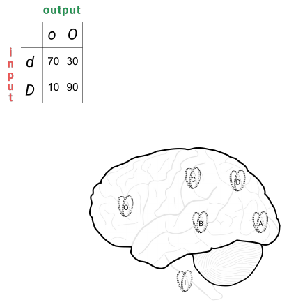
[The table now holds counts rather than single results: 70 (o) and 30 (O) in the d row, and 10 (o) and 90 (O) in the D row.]
To find the probabilities of the output state given the input states, we just normalize the rows (divide each element by the sum of the row).
If we see that some probabilities are indeed higher than chance, then we have reason to believe that D makes a difference to O, and we depict this with an arrow.
In the special case that the TPM is deterministic, all entries in the TPM would be 0 or 1, and there would be exactly one "1" per row.
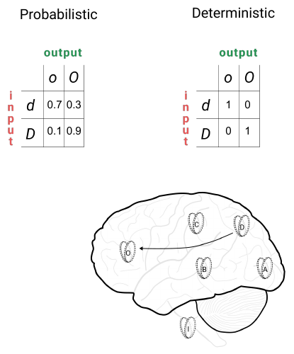
[Two tables stand side by side. The one labelled "Probabilistic" gives the normalized counts:
| input \ output | o (OFF) | O (ON) |
|---|---|---|
| d (OFF) | 0.7 | 0.3 |
| D (ON) | 0.1 | 0.9 |
The one labelled "Deterministic" shows the special case:
| input \ output | o (OFF) | O (ON) |
|---|---|---|
| d (OFF) | 1 | 0 |
| D (ON) | 0 | 1 |
Beneath the tables, the brain outline shows an arrow from D to O.]
The substrate graph (slides 25–26)
Some of the information in a TPM can also be represented visually in a substrate graph—a depiction of units with directed connections between them.
This very simple substrate graph indicates that the state of unit O depends on (or can take a difference from) the state of unit D.
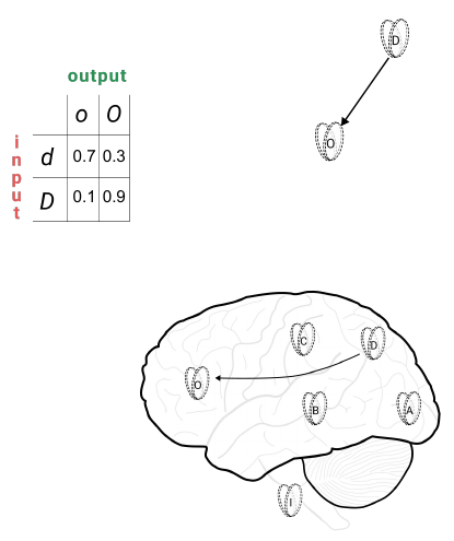
[Beside the D-to-O TPM, the substrate graph consists of just two unit icons, D and O, joined by a single arrow from D to O; the same arrow appears on the brain outline below.]
Self-loops (slides 27–28)
Note that we can also assess the cause–effect power of a single unit—its ability to take and make a difference from and to itself. This is indicated on a substrate graph as a self-loop.
Like any other arrow, the self-loop shows a direct causal constraint from some input to some output, as shown in the TPM. As before, we can determine the strength of the self-loop by setting the unit to all its available states and computing how likely it is to end up in each of its available states.
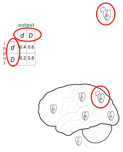
[Unit D is circled in red, both on the brain and in a small substrate graph showing D with a loop returning to itself. Its TPM has D as both input and output:
| input \ output | d (OFF) | D (ON) |
|---|---|---|
| d (OFF) | 0.4 | 0.6 |
| D (ON) | 0.2 | 0.8 |
| ] |
The substrate TPM (slides 29–32)
In IIT, we mostly use TPMs of many units at a time because we want to assess entire systems constituted of many units.
This substrate TPM (or system TPM) has all units both as inputs and outputs.
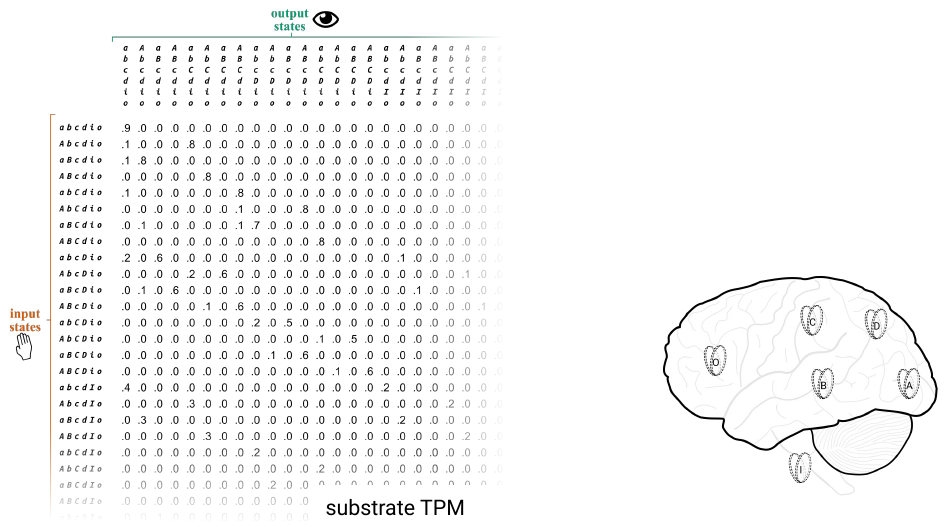
[The substrate TPM for the six units is shown as a large grid whose rows are all 64 input states (from abcdio to ABCDIO, marked "input states" with a hand icon) and whose columns are all 64 output states (marked "output states" with an eye icon). The entries are probabilities, most of them 0, and the lower rows and right-hand columns fade out to suggest that the table continues.]
As before, the TPM can be filled in by setting the input units into each of their possible states and recording the state of output units until we have a reliable estimate of all the conditional probabilities.
And, as before, we can represent the substrate in terms of connections among units.
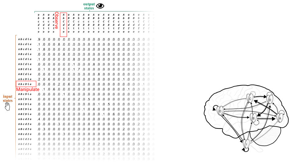
[In the substrate TPM, the input row AbcDio is boxed in red and labelled "Manipulate," and the output column AbCdio is boxed in red and labelled "Observe." On the brain outline, arrows of varying thickness now run in many directions among the six units, and several units have self-loops.]
Why substrate graphs are useful (slides 33–34)
However, the connections may become difficult to depict on the physical substrate itself—in this case, on the brain. This is where substrate graphs become an especially useful way to isolate and depict the causal connections of interest.
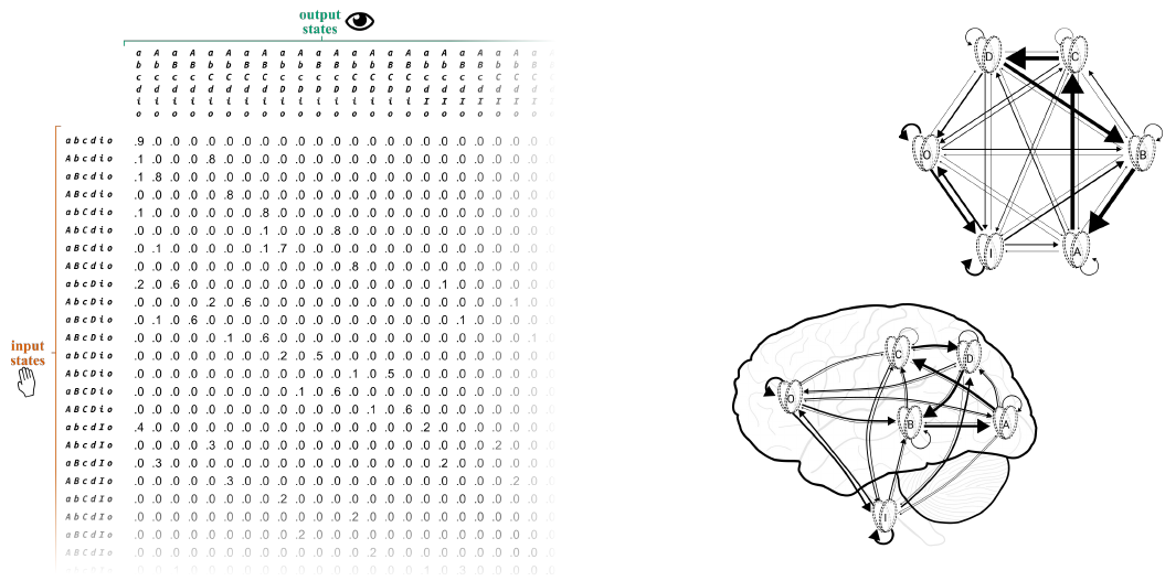
[The tangle of arrows on the brain outline is set beside a clean substrate graph in which the six units are arranged in a hexagon and every connection is drawn as a separate arrow.]
Reading a substrate graph (slides 35–36)
The substrate graph is a useful tool to get an intuitive understanding of the connections among units in the network.
In this example, every unit appears to be connected with every other one, and they all have self-loops. However, note that the strength of these connections varies considerably, as indicated by the thickness of the arrows (and sometimes by numbers).
To determine these connection strengths, we need to know a given unit's activation function, expressing the probability of a unit turning ON as a function of the sum of its input weights.
The substrate graph is used extensively in the IIT literature to indicate when specific operations are performed—especially pinning, partitioning, manipulating, and observing.
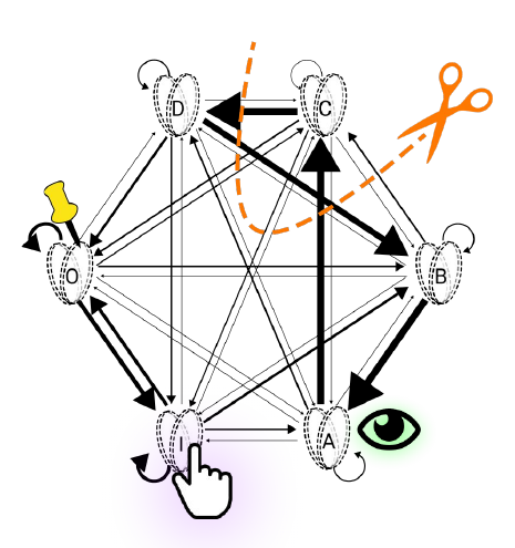
[The six units sit in a hexagon: D at top left, C at top right, B at right, A at bottom right, I at bottom left, and O at left. Every unit is connected to every other, and each has a self-loop; the arrows range from hairline to very thick, the thickest running from C to D, from D to B, from B to A, from A up to C, and between O and I. Four operations are marked on the graph, each in the colour used for its name in the text: a yellow pushpin on O (pinning); an orange pair of scissors with a dashed orange cut line that curves around unit C, separating it from the rest (partitioning); a purple hand pressing on I (manipulating); and a green eye watching A (observing).]
Summary slide (slide 37)
[The closing slide repeats the title slide (see slide 1 above), now labelled "summary": the substrate TPM, the single unit with its "observe" and "manipulate" icons, the substrate graph, and the brain outline labelled "substrate."]