# Slides: Computing Φ
*The lab's transcriptions of the decks embedded on https://www.iit.wiki/unfolding: each slide's text as the deck shows it, and in square brackets a description of each diagram, which is the transcriber's and not the deck's.*
## Slideshow 1: Unfolding - Apply intrinsicality - post Oct. 2023
Source page: [Computing Φ (technical)](https://www.iit.wiki/unfolding), step 2: Intrinsicality
Source deck: [Unfolding - Intrinsicality](https://docs.google.com/presentation/d/1FeugVnlCyNcZ0f3BKtAWBzCXjlvSdXgFxyhFSEYVo-g/edit) (94 slides)
### Title slide (slide 1)
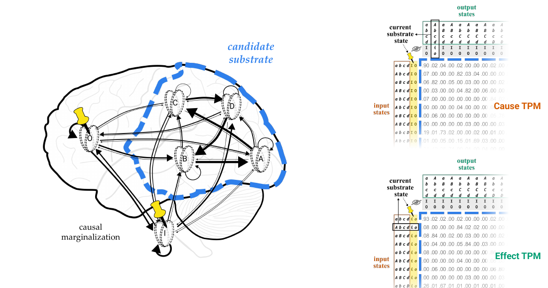
[On the left is the brain with the six units drawn as neuron-like icons. A dashed blue line, labelled "candidate substrate," encloses A, B, C and D; units I and O lie outside it, each with a yellow pushpin, under the label "causal marginalization." On the right are two 16-by-16 TPMs of the candidate system, one above the other: the "Cause TPM" (label in orange) and the "Effect TPM" (label in green). Each has the candidate's 16 states as input states down the side and output states across the top, and each shows the current substrate state, *Abcdio*, boxed in black: as an output column in the cause TPM and as an input row in the effect TPM. The background units' states are shaded yellow on the input side, with a small pushpin, and grey on the output side, with a crossed-out eye. A red "(click)" prompt invites the reader to advance.]
### Recap of the intrinsicality postulate (slides 2–5)
Recall from the [intrinsicality postulate](https://www.iit.wiki/axioms-and-postulates/intrinsicality#h.ffm1nm3ehxmu) that we aim to causally isolate a [candidate](https://www.iit.wiki/glossary#h.8mzotxp600xu) [substrate of consciousness](https://www.iit.wiki/glossary#h.j5clb514qcec) (e.g. **ABCD**).
We do this by causally marginalizing ("pinning") the [background units](https://www.iit.wiki/glossary#h.ot008m3n2clu) (e.g. **IO**) to render them causally inert.
This operation ensures that any remaining causal power must be *of and over the units* of the candidate substrate itself.
These slides focus on explaining what we do [operationally](https://www.iit.wiki/glossary#h.vztp822ktk99) when **marginalizing background units**.
These operations are necessary to let us **assess the cause–effect power from the intrinsic perspective** of the system.
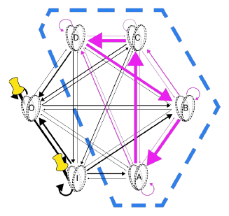
[The six-unit substrate graph, with units drawn as neuron-like icons, is shown with a dashed blue hexagon around A, B, C and D and yellow pushpins on O and I. The arrows among A, B, C and D, including their self-loops, are highlighted in magenta, showing the causal power that remains within the candidate; the connections to and from O and I stay black. On slides 2 and 3 the graph has no magenta highlighting. In the text, "pinning" is printed in yellow and "of and over the units" in magenta.]
### From one substrate TPM to two candidate TPMs (slides 6–9)
On the [TPM](https://www.iit.wiki/glossary#h.rgqyfluj1zit) representation from the [postulate](https://www.iit.wiki/axioms-and-postulates/intrinsicality#h.ffm1nm3ehxmu) (right), pinning was illustrated by applying yellow shading over the states of the background units on the **input** side, and gray shading on the **output** side (indicating that we ignore them).
This representation was good enough for the postulate, but imperfect because pinning operations result in two TPMs:
a **cause TPM** and an **effect TPM** (notice the numbers are slightly different).
These 4-unit TPMs will be used throughout the remaining postulates. This slide deck, however, aims to show how the 4-unit TPMs are "condensed" out of the original 6-unit substrate TPM.
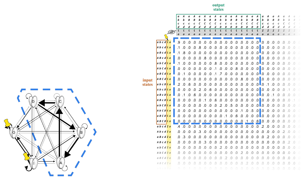
[Beside the substrate graph is the substrate TPM from the Intrinsicality Postulate deck, with the 64 input states of ABCDIO down the side and the output states across the top. The block of entries for the candidate is outlined in dashed blue. On the input side, the letters for I and O in the row labels are shaded yellow and marked with a small pushpin; on the output side, the rows of column labels for I and O are shaded grey and marked with a crossed-out eye. On slide 8 this table is replaced by the two 16-by-16 TPMs, cause and effect.]
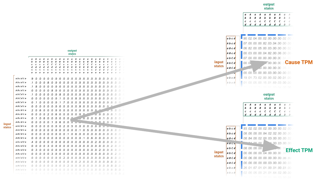
[The substrate TPM appears again at left, without the pinning shading, and two large grey arrows lead from it to the cause TPM (label in orange) and to the effect TPM (label in green) at right, showing that both 4-unit TPMs are condensed out of the one 6-unit TPM.]
### Conditioning on the current state (slides 10–16)
In technical terms, we [causally marginalize](https://www.iit.wiki/glossary#h.vq8lj719uzmz) out the background units (**I** and **O**) by conditioning on the **current state** of the substrate.
In the [postulates sequence](https://www.iit.wiki/axioms-and-postulates#h.8d1ocowludyo), we only introduced the current state of the substrate in the information postulate, highlighting the property of *specificity*. Operationally, however, we must use our knowledge of the current state (***Abcdio***) already in this intrinsicality step to guide how we marginalize units **I** and **O** out of each TPM.
Hence these TPMs are specific to current substrate state ***Abcdio***. In the **cause TPM**, the current state is considered an output, while in the **effect TPM**, it is considered an input.
We illustrate causal marginalization by "pinning" background units on the input side (yellow) and ignoring them (gray) on the output side.
Before getting into details…
This black box indicates that we know this to be the *current* substrate state—not only of our candidate (***Abcd***) but also of our background units (***io***).
This knowledge of the current substrate state affects how we pin background units in their possible input states—that is, we take a *weighted* average of their possible states.
In contrast, the grayed-out **IO** indicates that we ignore the possible output states of these units—that is, we sum the probabilities associated with any particular state of A, B, C, and D over all possible states of I and O.
Now let's see the operational details for obtaining each TPM.
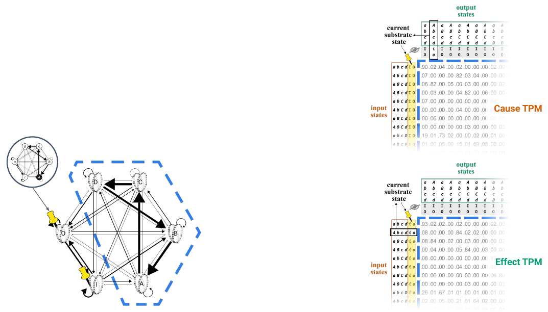
[On the left is the substrate graph, with ABCD enclosed in dashed blue and I and O pinned; a small circular inset at upper left shows the same graph in its current state, with A ON and the other units OFF. On the right, each TPM now carries two extra label rows for I and O. In the cause TPM, the current substrate state *Abcdio* is boxed in black as an output column headed "current substrate state"; in the effect TPM, it is boxed as an input row. The columns for I and O on the input side are shaded yellow, and their rows on the output side are shaded grey. On slides 14–16, callout boxes point to the black box, to the yellow input shading and to the grey output shading with the three sentences given above.]
### The effect TPM: state-by-state and state-by-node (slides 18–23)
We'll start with the **effect TPM** since it's a bit simpler.
Again, our goal is to "condense" the effect TPM from the big substrate TPM, shown here as a state-by-**state** TPM.
But to understand the transformations required, it will be more convenient to use a [state-by-**node**](https://www.iit.wiki/glossary#h.clm375b2y9cx) TPM instead (as generated by [PyPhi](https://centerforsleepandconsciousness.psychiatry.wisc.edu/pyphi-software/), using a heat map instead of numbers).
This indicates the system input state (ABCDIO) with 0 = OFF, 1 = ON. (We'll zoom in shortly.)
And the heatmap indicates the probability of the respective node turning ON given the system input state.
Since we ignore units **I** and **O** in the output of the effect TPM, we can simply ignore these two columns for now.
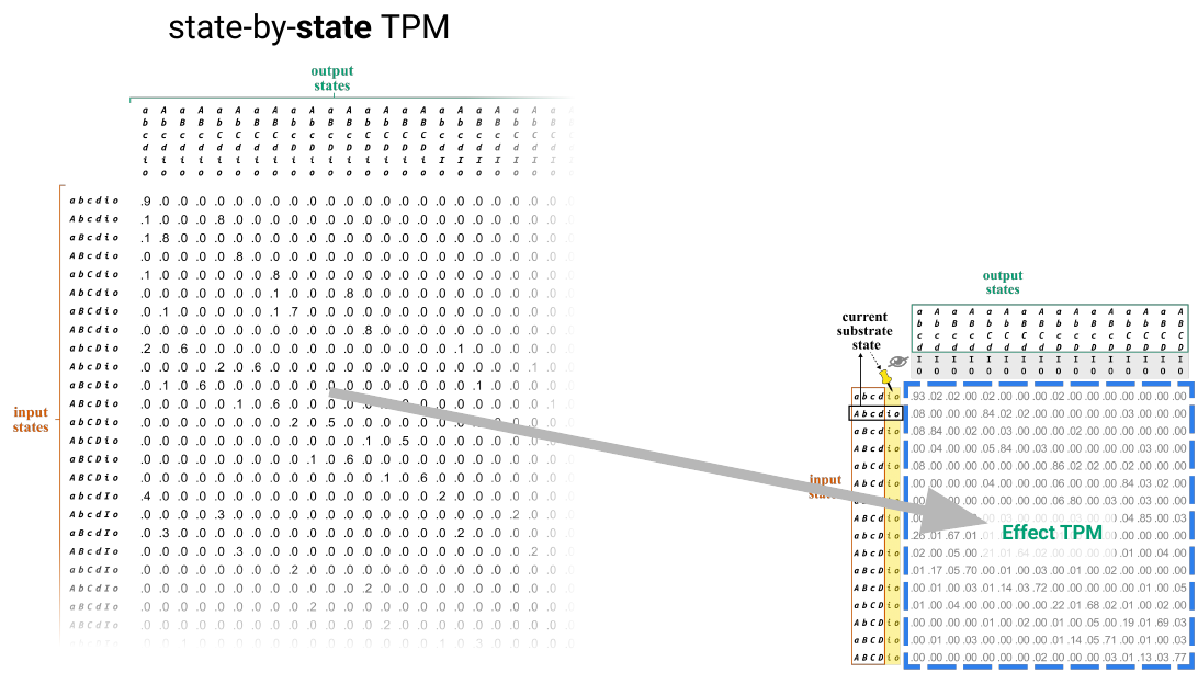
[At left, headed "state-by-state TPM," is the substrate TPM with all 64 input states (from *abcdio* down) and all 64 output states, most entries 0 and a few near 1. A large grey arrow leads from it to the 16-by-16 effect TPM at right.]
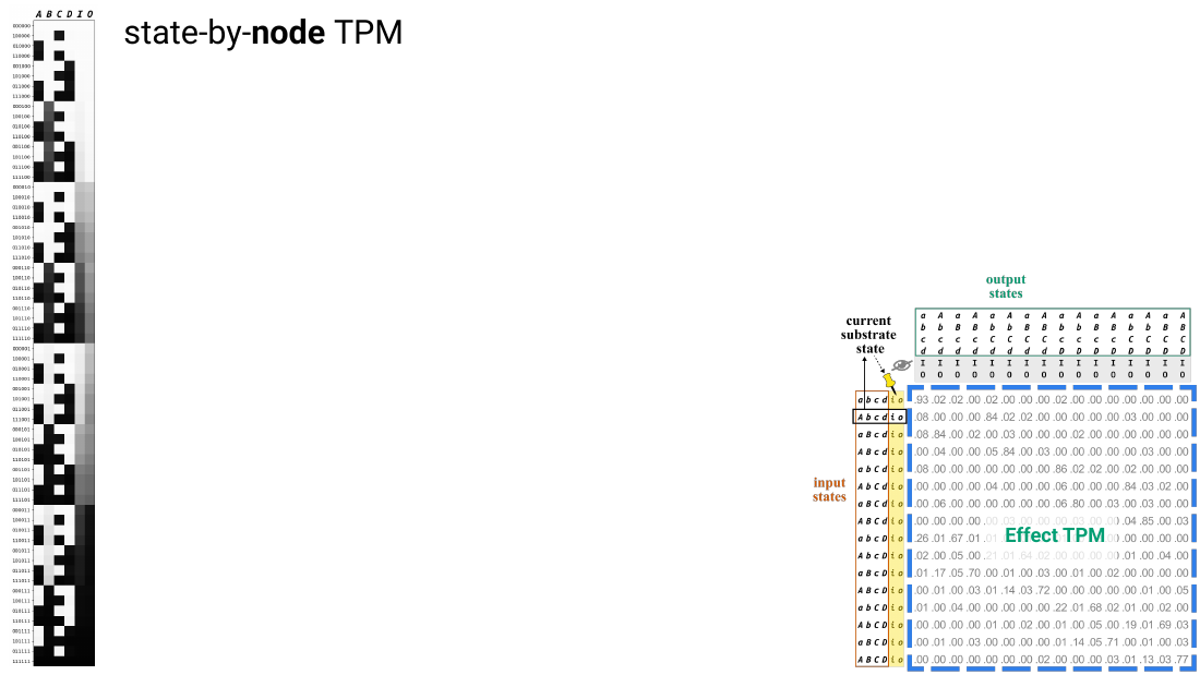
[From slide 20 onward the state-by-state TPM is replaced, at the left edge of the slide, by a tall, narrow "state-by-node TPM": 64 rows, one per input state of ABCDIO written as a string of 0s and 1s (for example 000000 for *abcdio* and 100000 for *Abcdio*), and six columns headed A, B, C, D, I and O. Each cell is a grey level from white (probability near 0 that the unit turns ON) to black (near 1). On slide 21, callout boxes point to the row labels and to the heat map with the two sentences given above; on slides 22 and 23, the columns for I and O are shaded and then removed.]
### Dividing the state-by-node TPM into blocks (slides 24–26)
It will be useful to divide up our TPM into "blocks" according to the state of the background units.
Since the current state (***Abcdio***) is on the input side, this block is the only relevant one to look at (in other words, the block with **I** and **O** both OFF).
This is also depicted on the effect TPM, where the background units have been "pinned" in their current state ***io***.
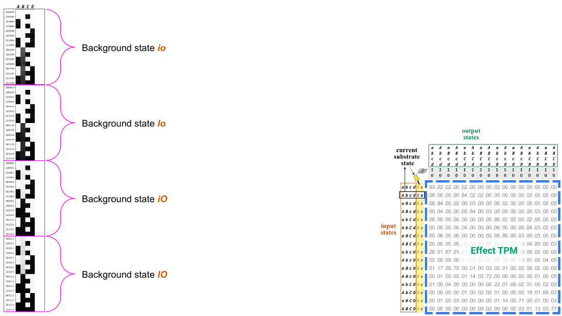
[Magenta braces divide the 64 rows of the state-by-node TPM into four blocks of 16 rows, labelled "Background state *io*," "Background state *Io*," "Background state *iO*" and "Background state *IO*." The effect TPM is shown at right. On slides 25 and 26, callout boxes point to the first block, *io*, and to the pinned *io* in the effect TPM with the two sentences given above.]
### Zooming in on the block with background state io (slides 27–30)
We can therefore "zoom in" on this block and ignore the rest: these rows show the probability that each unit in the candidate system is turned **ON** (gray columns) by every possible state of **ABCD** with background units ***io*** (rows).
P(**X=ON** | **Y=ABCD*io***)
This reads as "the probability unit X as **output** will turn ON given substrate state Y as **input**."
Recall that we use roman uppercase to refer to units generically, and italic uppercase for ON and italic lowercase for OFF.
These are all the probabilities we need to compute the effect TPM.
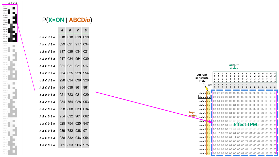
[The first 16 rows of the state-by-node TPM, outlined in magenta at the left edge, are enlarged into a table headed "P(X=ON | ABCD*io*)." A magenta line connects the table to the effect TPM at right. The table reads:
| input state | A | B | C | D |
|---|---|---|---|---|
| *abcdio* | .018 | .018 | .018 | .018 |
| *Abcdio* | .029 | .021 | .917 | .034 |
| *aBcdio* | .917 | .029 | .034 | .021 |
| *ABcdio* | .947 | .034 | .954 | .039 |
| *abCdio* | .021 | .021 | .021 | .917 |
| *AbCdio* | .034 | .025 | .928 | .954 |
| *aBCdio* | .928 | .034 | .039 | .928 |
| *ABCdio* | .954 | .039 | .961 | .961 |
| *abcDio* | .021 | .723 | .021 | .029 |
| *AbcDio* | .034 | .754 | .928 | .053 |
| *aBcDio* | .928 | .808 | .039 | .034 |
| *ABcDio* | .954 | .832 | .961 | .062 |
| *abCDio* | .025 | .754 | .025 | .947 |
| *AbCDio* | .039 | .782 | .938 | .971 |
| *aBCDio* | .938 | .832 | .046 | .954 |
| *ABCDio* | .961 | .853 | .966 | .975 |
Each entry is the probability that the unit heading the column is ON after one update, given the input state of the row. The remaining 48 rows of the state-by-node TPM are greyed out. On slides 28 and 29, callout boxes carry the two sentences on how to read the notation.]
### Computing the first row of the effect TPM (slides 31–41)
From the top row of the state-by-node TPM, we can compute the upper-left probability (0.93) in the effect TPM.
First, we need to know the probabilities that each unit will be OFF (not just ON) after the transition.
Because the units are binary, this probability is found by simple subtraction: P(OFF) = 1 – P(ON).
| | |
|---|---|
| P(*a*\|*abcdio*) = 1 – P(*A*\|*abcdio*) | 0.982 |
| P(*b*\|*abcdio*) = 1 – P(*B*\|*abcdio*) | 0.982 |
| P(*c*\|*abcdio*) = 1 – P(*C*\|*abcdio*) | 0.982 |
| P(*d*\|*abcdio*) = 1 – P(*D*\|*abcdio*) | 0.982 |
And because the units are conditionally independent, we can now find the probability in the effect TPM by multiplying together the unit-wise probabilities we just obtained.
P(*abcd* | *abcdio*) = 0.982 * 0.982 * 0.982 * 0.982 ≈ 0.93
Note that this is the corresponding formula in [IIT 4.0](https://journals.plos.org/ploscompbiol/article?id=10.1371/journal.pcbi.1011465), which relates probabilities in the substrate TPM to the effect TPM.
$$\mathcal{T}_e = \mathcal{T}_e(\mathcal{T}_U, u, w) \equiv p_e(\bar{s} \mid s) = p(\bar{s} \mid s, w), \quad s, \bar{s} \in \Omega_S$$
Here, *u* refers to the current state of the substrate, *w* to the state of the background conditions; *s* and s̄ are the current and output states of the candidate complex, respectively.
We can do the same thing for the transition ***abcd*** to ***Abcd*** by multiplying the relevant probabilities obtained from the state-by-node TPM.
P(*Abcd* | *abcdio*) = 0.018 * 0.982 * 0.982 * 0.982 ≈ 0.02
…and for ***abcd*** to ***aBcd***, ***abcd*** to ***ABcd***, ***abcd*** to ***abCd***, and so on till the end of the first row.
P(*aBcd* | *abcdio*) = 0.982 * 0.018 * 0.982 * 0.982 ≈ 0.02
P(*ABcd* | *abcdio*) = 0.018 * 0.018 * 0.982 * 0.982 ≈ 0.00
P(*abCd* | *abcdio*) = 0.982 * 0.982 * 0.018 * 0.982 ≈ 0.00
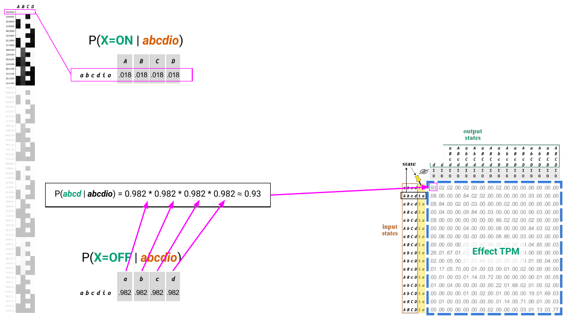
[At top, "P(X=ON | *abcdio*)" shows the first row of the table, .018 for each of A, B, C and D. At bottom, "P(X=OFF | *abcdio*)" shows the complementary row, .982 for each of *a*, *b*, *c* and *d*. Four magenta arrows lead from the OFF probabilities into the equation "P(*abcd* | *abcdio*) = 0.982 * 0.982 * 0.982 * 0.982 ≈ 0.93," and a magenta line leads from the equation to the top-left entry of the effect TPM. On slides 37–40, the arrows are redrawn for each transition, taking the ON probability (.018) for each unit that is ON in the output state and the OFF probability (.982) for each unit that is OFF.]
### The remaining rows (slides 42–43)
The second row in the effect TPM can be computed in the same way using the second row of the state-by-node TPM.
…and so on for all the possible system input states.
[On slide 42, the second row of the table, P(X=ON | *Abcdio*) = .029, .021, .917, .034, is outlined and linked to the second row of the effect TPM; on slide 43, the whole table is outlined and linked to the whole effect TPM.]
### Why the cause TPM is harder (slides 44–47)
To recap, when computing the **effect TPM**, our knowledge of the current substrate state fully determines the relevant background conditions—units **I** and **O** were in state ***io*** with 100% certainty. This made it straightforward to marginalize out the causal contribution of the background units.
Unfortunately, when computing the **cause TPM**, it's (usually) not possible to divide the state-by-node TPM into blocks of relevant and irrelevant input states.
This is because the current state is now on the output side; thus the background conditions are not directly "inherited" from the substrate state.
And we now depict the input states of I and O as variable.
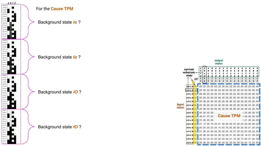
[The state-by-node TPM is again divided into four blocks, now labelled "Background state *io* ?," "Background state *Io* ?," "Background state *iO* ?" and "Background state *IO* ?" under the heading "For the Cause TPM." The cause TPM is shown at right, with the current substrate state boxed as an output column. On slide 44, under "For the Effect TPM," only the *io* block is bright and the other three are faded. On slides 46 and 47, callout boxes carry the two sentences given above.]
### The probability of each background condition (slides 48–51)
Still, it is possible to find a *probability distribution* of the background conditions by using our knowledge of the current substrate state: P(**IO** | ***Abcdio***).
Notice it's black because this refers to the the actual current state (not a counterfactual state).
That is, by "back-propagating" the knowledge of the current substrate state "through" the substrate TPM (using Bayes' rule), we find the probability of each possible background condition (***io***, ***Io***, ***iO***, or ***IO***) given the current substrate state.
We can then use the resulting probabilities to help us marginalize out the background units to yield the cause TPM.
| | |
|---|---|
| P(*io* \| ***Abcdio***) | 0.559 |
| P(*Io* \| ***Abcdio***) | 0.192 |
| P(*iO* \| ***Abcdio***) | 0.245 |
| P(*IO* \| ***Abcdio***) | 0.004 |
So as not to interrupt the flow, we have simply given the respective probabilities here. But we will return to how they're calculated at the end of this sequence (slide 80).
### Computing the cause TPM (slides 52–69)
Again, let's work through some examples computing the cause TPM from the state-by-node substrate TPM, starting with the top-left probability (0.90).
Just like for the effect TPM, the cause TPM probability is obtained by taking a product of probabilities computed from rows of the full substrate TPM.
P(*abcd* | *abcd*) = P(*a* | *abcd*) * P(*b* | *abcd*) * P(*c* | *abcd*) * P(*d* | *abcd*) ≈ 0.90
However, we can no longer look at just one row of the state-by-node TPM but will have to pull from **multiple rows**. This is because **I** and **O** may have been ON or OFF in the input state (even though they are both OFF in the current state).
For example, this is the probability of ***a*** in the output given ***abcd*** in the input.
But input state ***abcd*** can appear in any combination with units **I** and **O**.
So to look at ***abcd*** alone, we have to "collapse" these four rows of probabilities into this single probability.
In technical terms, to marginalize out the causal contribution of units **I** and **O**, we need to renormalize the probabilities and sum across the possible states of **I** and **O** before taking the product.
This means we first multiply each state-by-node probability by these **factors**…
As shown before (slide 50), these are the probabilities of each input state of **IO** (***io***, ***Io***, ***iO***, or ***IO***) given the specific current state of the whole substrate (***Abcdio***).
…in order to get the **renormalized probabilities**.
We then **sum the columns** to obtain the probabilities that each unit turns **ON**, given the input state ***abcd*** with **I** and **O** marginalized out.
Like for the effect TPM, we then need to compute the probabilities of each unit being OFF given input state ***abcd***. Again, since these are binary units, P(**OFF** | ***abcd***) is simply 1 – P(**ON** | ***abcd***).
Finally, we are able to take the product of the P(**OFF** | ***abcd***) probabilities to calculate the top-left value in the cause TPM.
P(*abcd* | *abcd*) = 0.977 * 0.962 * 0.971 * 0.981 ≈ 0.90
We can now follow the same pattern as for the effect TPM to compute the transition probability to ***Abcd***, to ***aBcd***, to ***ABcd***, and so on for all states resulting from the input state ***abcd***.
P(*Abcd* | *abcd*) = 0.023 * 0.962 * 0.971 * 0.981 ≈ 0.02
P(*aBcd* | *abcd*) = 0.977 * 0.038 * 0.971 * 0.981 ≈ 0.04
P(*ABcd* | *abcd*) = 0.023 * 0.038 * 0.971 * 0.981 ≈ 0.00
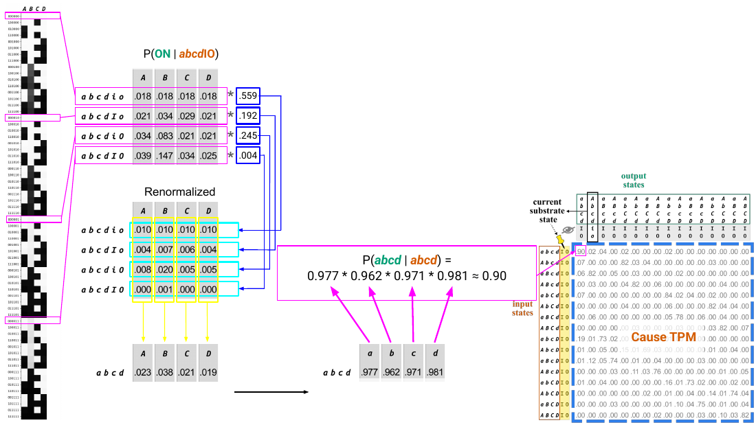
[Four rows of the state-by-node TPM, one from each background block, are outlined in magenta and enlarged into a table headed "P(ON | *abcd*IO)." Each row is multiplied by its factor, shown in a blue box, to give a "Renormalized" table; yellow boxes around each column lead down to the column sums; and the sums are turned into OFF probabilities and multiplied, as the equation that feeds the top-left entry of the cause TPM at right. The numbers are:
| input state | A | B | C | D | factor |
|---|---|---|---|---|---|
| *abcdio* | .018 | .018 | .018 | .018 | × .559 |
| *abcdIo* | .021 | .034 | .029 | .021 | × .192 |
| *abcdiO* | .034 | .083 | .021 | .021 | × .245 |
| *abcdIO* | .039 | .147 | .034 | .025 | × .004 |
| renormalized | A | B | C | D |
|---|---|---|---|---|
| *abcdio* | .010 | .010 | .010 | .010 |
| *abcdIo* | .004 | .007 | .006 | .004 |
| *abcdiO* | .008 | .020 | .005 | .005 |
| *abcdIO* | .000 | .001 | .000 | .000 |
| **sum: P(ON \| *abcd*), I and O marginalized out** | **.023** | **.038** | **.021** | **.019** |
| | *a* | *b* | *c* | *d* |
|---|---|---|---|---|
| P(OFF \| *abcd*), I and O marginalized out | .977 | .962 | .971 | .981 |
On slides 66–68, magenta arrows pick out the ON probability for each unit that is ON in the output state and the OFF probability for each unit that is OFF, for the transitions to *Abcd*, *aBcd* and *ABcd*.]
### The formula in IIT 4.0 (slides 70–79)
While this might seem complicated, the main point is that any contribution of the background units can be **marginalized** out by using the knowledge of the current substrate state to **renormalize** the system's state transition probabilities.
These steps are explicitly formalized in [IIT 4.0, formula (4)](https://journals.plos.org/ploscompbiol/article?id=10.1371/journal.pcbi.1011465#sec025):
$$\mathcal{T}_c = \mathcal{T}_c(\mathcal{T}_U, u, w) \equiv p_c(s \mid \bar{s}) = \prod_{i=1}^{|S|} \sum_{\bar{w}} p(s_i \mid \bar{s}, \bar{w}) \left( \frac{\sum_{\hat{s}} p(u \mid \hat{s}, \bar{w})}{\sum_{\hat{u}} p(u \mid \hat{u})} \right), \quad s, \bar{s} \in \Omega_S$$
Let's briefly illustrate by revisiting how we got the first TPM square.
the **probability** of a transition from an **input state** (s̄) to an **output state** (s) is given by the **product** of **renormalized probabilities**, dependent on the current substrate state **u**, **summed** over all possible background unit states (w̄).

[Over slides 73–79, each part of the formula is boxed in turn, in the colour in which the sentence highlights the words that name it: red for the probability pc(s | s̄), orange for the input state s̄, green for the output state s, black for the product over units, cyan for the renormalization factor, green for the current substrate state u (in both numerator and denominator), and yellow for the sum over background states w̄. On slide 72, a callout box carries the sentence about revisiting the first TPM square.]
### Where the renormalization factors come from (slides 80–90)
Finally, let's return to where the renormalization factors came from.
In brief, they are given by this…but let's unpack it a little.
$$\frac{\sum_{\hat{s}} p(u \mid \hat{s}, \bar{w})}{\sum_{\hat{u}} p(u \mid \hat{u})}$$
This factor represents the probability that a particular state of **I** and **O** (w̄) was present as an input leading to the current state of the substrate (u).
And the probabilities required can be read off of the state-by-state TPM.
The **numerator** quantifies the sum of probabilities for transitions to the current substrate state (u; here ***Abcdio***) from all possible system (input) states (ŝ) given a particular background state (w̄; here, ***io***).
Similarly, the **denominator** quantifies the sum of probabilities for transitions to the current substrate state (u; here ***Abcdio***) from *any possible input state* of the full substrate (û).
Thus, the factor quantifies the probability of transitioning to the current substrate state from a state with a particular background condition, relative to the overall probability of transitioning there at all.
In essence, this computation amounts to finding the probabilities of transitioning backwards *from* an output state to an input state by applying Bayes' rule to the forwards probabilities (in the TPM) assuming a uniform prior over the input states.
For the background condition ***io***, the computation becomes:
P(*io* | ***Abcdio***) = 1.084 / 1.939 = 0.559.
This is the same value we saw before.
In the same way, we can compute the renormalization factor for all other possible background conditions (***Io***, ***iO***, and ***IO***).
P(*Io* | ***Abcdio***) = 0.372 / 1.939 = 0.192.
P(*iO* | ***Abcdio***) = 0.476 / 1.939 = 0.245.
P(*IO* | ***Abcdio***) = 0.008 / 1.939 = 0.004.
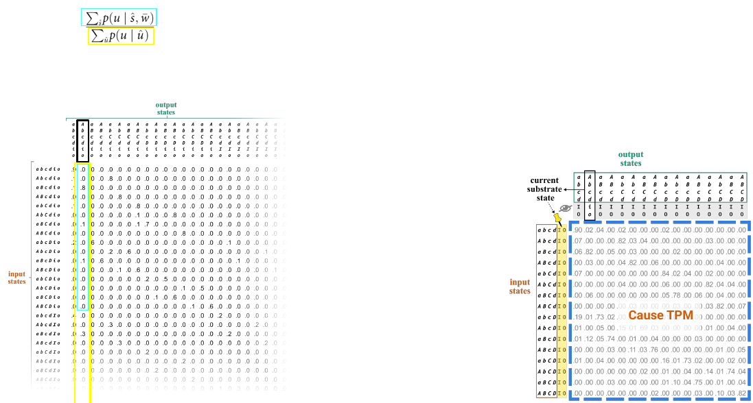
[At top left is the renormalization factor, with the numerator boxed in cyan and the denominator in yellow. Below it is the 64-state state-by-state TPM with the column for the current substrate state, *Abcdio*, boxed in black. The entries of that column in the 16 rows with background state *io* are outlined in cyan (their sum is the numerator, 1.084), and the whole column is outlined in yellow (its sum over all 64 input states is the denominator, 1.939). The entries shown are rounded to one decimal place. The cause TPM is shown at right. On slide 88, the numbers 1.084 and 1.939 are highlighted in the same colours in the equation.]
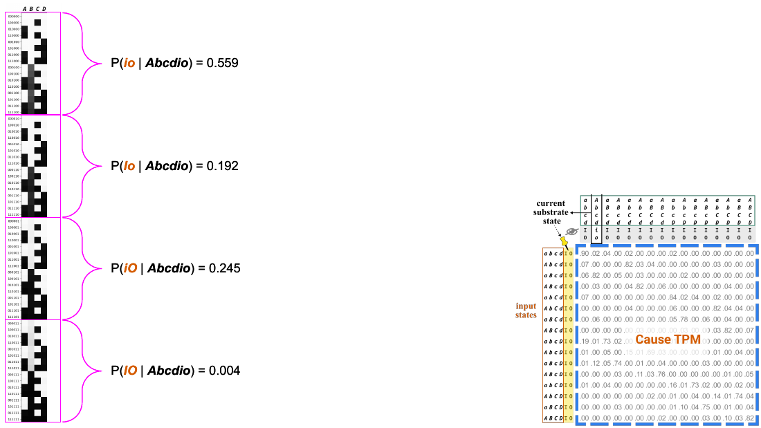
[The state-by-node TPM is divided by magenta braces into its four blocks, now labelled with their probabilities: P(*io* | *Abcdio*) = 0.559, P(*Io* | *Abcdio*) = 0.192, P(*iO* | *Abcdio*) = 0.245 and P(*IO* | *Abcdio*) = 0.004. The cause TPM is shown at right.]
### The two TPMs (slides 91–93)
Now we have our two TPMs.
For simplicity's sake, we will drop the background units from the TPM illustrations for the remaining operational steps.
With these TPMs in hand, we are in a position to assess the **intrinsic cause–effect power** from the **perspective of the system** in its current state. These notions will be operationalized in the next step of computing *intrinsic information*.
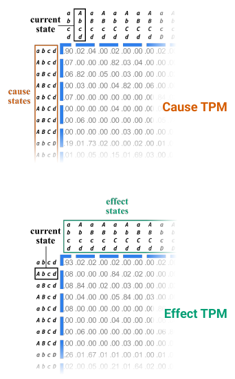
[The cause TPM (label in orange, rows marked "cause states") and the effect TPM (label in green, columns marked "effect states") are shown one above the other, now with only the four candidate units in their row and column labels and the current state *Abcd* boxed in black: as a column in the cause TPM and as a row in the effect TPM. The first row of the cause TPM begins .90, .02, .04, .00, .02; the first row of the effect TPM begins .93, .02, .02, .00, .02; the current-state row of the effect TPM contains .84 under *abCd*.]
### Summary slide (slide 94)
[The closing slide, labelled "summary," repeats the diagram from slide 1: the brain with the candidate substrate enclosed in dashed blue and the background units I and O pinned under the label "causal marginalization," beside the finished cause TPM and effect TPM.]
## Slideshow 2: Unfolding - information
Source page: [Computing Φ (technical)](https://www.iit.wiki/unfolding), step 3: Information
Source deck: [Unfolding - information](https://docs.google.com/presentation/d/1zn8ljJ6vGhz_m81HbEnWa5twq3JPob6guP-DBSBIcxw/edit) (26 slides)
### Title slide (slide 1)
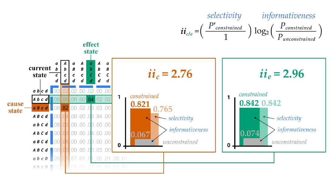
[At top right is the formula for intrinsic information, with its two factors labelled "selectivity" and "informativeness":
$$ii_{c/e} = \left( \frac{P'_{\text{constrained}}}{1} \right) \log_2 \left( \frac{P_{\text{constrained}}}{P_{\text{unconstrained}}} \right)$$
At left is the TPM of the candidate system, with the current state *Abcd* boxed in black, the cause state *aBcd* marked in orange (entry .82) and the effect state *abCd* in green (entry .84). Lines lead from the TPM to two bar charts, each on an axis from 0 to 1. The orange chart, headed "*ii*c = 2.76," has a tall orange bar labelled "constrained" (0.821), a paler bar beside it labelled "selectivity" (0.765), and a short grey bar labelled "unconstrained" (0.067); the gap between the constrained and unconstrained bars is labelled "informativeness." The green chart, headed "*ii*e = 2.96," has a green constrained bar (0.842), a paler selectivity bar of the same height (0.842), and a grey unconstrained bar (0.074). A red "(click)" prompt invites the reader to advance.]
### Finding the cause–effect state (slides 2–5)
Recall from the [information postulate](https://www.iit.wiki/axioms-and-postulates/information#h.lnlbeg807l4) that we aim to find the specific [cause–effect state](https://www.iit.wiki/glossary#h.tp4brteczc2p) of the system in its current state.
To do this, we need to calculate the intrinsic information (*ii*) for every possible cause state (red column) and effect state (green row). And by the [principle of maximal existence](https://www.iit.wiki/glossary#h.qof4052teerl), we choose the cause and effect states for which *ii* is maximal.
Here, we will demonstrate how *ii* is calculated by using the final, maximal cause–effect state as our example (***aBcd***–***abCd***).
We will start with calculating the effect state, which means we treat the **current state** as our input and the **effect state** as our output.
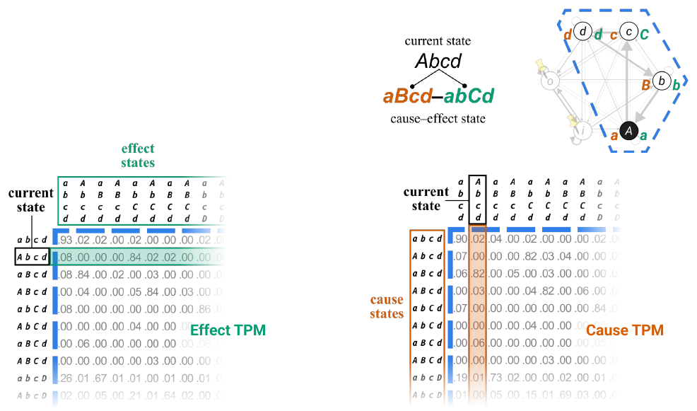
[At top, "current state *Abcd*" leads to "*aBcd*–*abCd*, cause–effect state," beside the substrate graph with each candidate unit's cause state in orange and effect state in green. Below are the two TPMs. In the effect TPM (label in green), the current state *Abcd* is boxed as an input row, and that whole row, together with the column headings above it, is outlined and shaded in green: these are all the possible effect states. In the cause TPM (label in orange), the current state is boxed as an output column, and that whole column, together with the row labels beside it, is outlined and shaded in orange: these are all the possible cause states.]
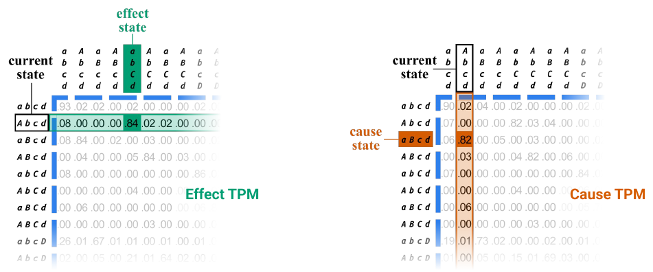
[The same two TPMs, now with a single state picked out in each. In the effect TPM, the column for the effect state *abCd* is shaded green and labelled "effect state," and its entry in the current-state row, .84, is highlighted. In the cause TPM, the row for the cause state *aBcd* is shaded orange and labelled "cause state," and its entry in the current-state column, .82, is highlighted. On slide 5 the cause TPM is removed.]
### The effect side: constrained and unconstrained probability (slides 6–10)
To calculate *ii* for the effect state, we will use two different probabilities:
- **Constrained** probability: this is the probability of a specific effect state given that the system is set to its specific current state. In other words, it's the number we read off the [effect TPM](https://www.iit.wiki/glossary#h.rgqyfluj1zit) (which varies slightly here due to rounding).
- **Unconstrained** probability: this is the average probability of that effect state if the system is initialized in all possible states.
**Unconstrained** probability:
P = (0.02 + 0.84 + 0.00 + 0.05 + …) / *N*, where *N* is the number of possible input states
P = (0.02 + 0.84 + 0.00 + 0.05 + …) / 16 = 0.074
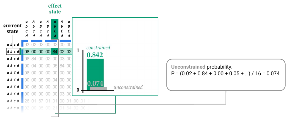
[Beside the effect TPM is a bar chart framed in green, on an axis from 0 to 1. A tall green bar labelled "constrained" shows 0.842, the entry for *abCd* in the current-state row. A short grey bar labelled "unconstrained" shows 0.074. In the TPM, the whole column for *abCd* is outlined in grey, and a line leads from it to a callout box giving the calculation of the unconstrained probability as the average of that column over all 16 input states. On slide 6 the chart is empty; on slide 7 only the constrained bar is drawn.]
### Informativeness and selectivity on the effect side (slides 11–14)
These values are used to calculate our *informativeness* factor, which we can crudely think of as the "raw power" of the system in its current state over a specific effect state.
On the effect side, we also use our constrained probability as our *selectivity* factor, which measures how much the system's [cause–effect power](https://www.iit.wiki/glossary#h.vlk7u52cim8x) is concentrated over a specific effect state. We can crudely think of selectivity as the system's "control" over its effect state, which attenuates its "raw power" over that state (its *informativeness*).
We denote this with P' because, for the cause-side computation, it will be different from the P in the informativeness factor.
$$ii_e = \left( \frac{P'_{\text{constrained}}}{1} \right) \log_2 \left( \frac{P_{\text{constrained}}}{P_{\text{unconstrained}}} \right)$$
$$2.96 = \left( \frac{0.842}{1} \right) \log_2 \left( \frac{0.842}{0.074} \right)$$
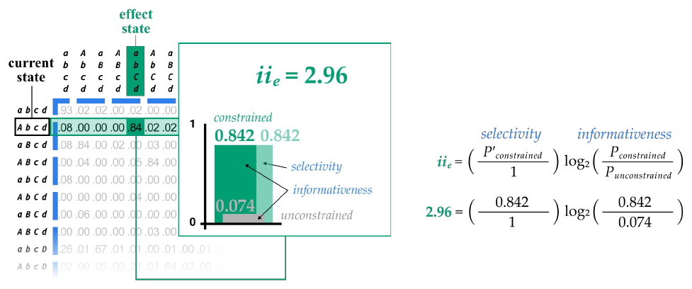
[The green bar chart, now headed "*ii*e = 2.96," shows the constrained bar (0.842), a paler bar of the same height beside it labelled "selectivity" (0.842), and the unconstrained bar (0.074), with the gap between constrained and unconstrained labelled "informativeness." To the right, the formula is written with its two factors labelled "selectivity" and "informativeness," and below it the same formula with the numbers substituted. On slide 11 only the informativeness factor is shown, as log2(0.842 / 0.074); on slide 13, a callout box carries the sentence about P'.]
### The cause side: constrained and unconstrained probability (slides 15–20)
To calculate *ii* for the cause state, we now treat the **cause state** as the input and the **current state** as the output.
Note that the TPM numbers have changed slightly because we are now using the cause TPM, as explained in the [intrinsicality step](https://www.iit.wiki/unfolding#h.5qi5tc64lye6).
Like for the effect state, we use the constrained and unconstrained probabilities to calculate our *informativeness* factor.
As before, the constrained probability is read off of the cause TPM directly.
And, again, we calculate the unconstrained probability by averaging over the whole column associated with the cause state. This gives us the probability of *transitioning to* the current state, independent of cause states—it is the probability of ending up in the current state, *unconstrained* by the specific cause state.
**Unconstrained** probability:
P = (0.02 + 0.00 + 0.82 + 0.03 + …) / 16 = 0.067
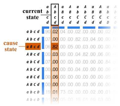
[The cause TPM, with the current state *Abcd* boxed as an output column and that column shaded orange. The row for the cause state *aBcd* is shaded orange and labelled "cause state," and its entry in the current-state column, .82, is highlighted. Reading down the current-state column, the entries begin .02 (from *abcd*), .00 (*Abcd*), .82 (*aBcd*), .03 (*ABcd*), .00, .00, .06, .00, .01.]
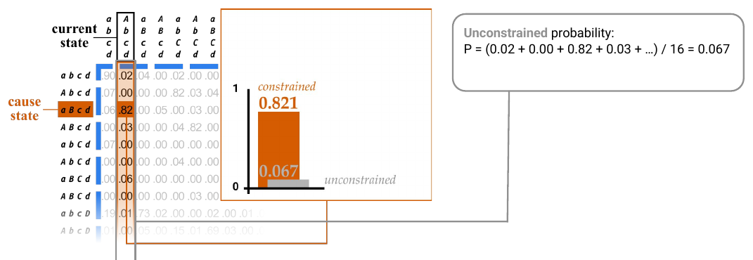
[Beside the cause TPM is a bar chart framed in orange, on an axis from 0 to 1. A tall orange bar labelled "constrained" shows 0.821, and a short grey bar labelled "unconstrained" shows 0.067. The whole current-state column of the TPM is outlined, and a line leads from it to a callout box giving the calculation of the unconstrained probability as the average of that column over all 16 cause states. On slide 17 the chart is empty; on slides 18 and 19 only the constrained bar is drawn.]
### Selectivity on the cause side (slides 21–25)
But unlike before, the *selectivity* factor is not simply taken as the constrained probability, which is why it is marked by P'.
This is because we must "take the perspective" of the current state to quantify the cause information it specifies. We can imagine this as "looking backward" from the current state to consider what the most-likely cause must have been.
Hence, we use the "backward" probability found by applying Bayes' rule to the "forward" probabilities in the cause TPM, which yields P' (see [this FAQ](https://www.iit.wiki/faqs/technical#h.uj8qdrmujwi) for more)
$$ii_c = \left( \frac{P'_{\text{constrained}}}{1} \right) \log_2 \left( \frac{P_{\text{constrained}}}{P_{\text{unconstrained}}} \right)$$
$$2.76 = \left( \frac{0.765}{1} \right) \log_2 \left( \frac{0.821}{0.067} \right)$$
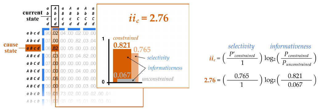
[The orange bar chart, now headed "*ii*c = 2.76," shows the constrained bar (0.821), a paler, shorter bar beside it labelled "selectivity" (0.765), and the unconstrained bar (0.067), with the gap between constrained and unconstrained labelled "informativeness." Unlike on the effect side, the selectivity bar is lower than the constrained bar. To the right, the formula is written with its factors labelled "selectivity" and "informativeness," and below it the same formula with the numbers substituted. On slide 21 only the informativeness factor is shown, as log2(0.821 / 0.067).]
### Summary (slide 26)
As a final note, recall that these steps have to be performed for every possible cause state (red column) and effect state (green row) of the system in its current state. Only then can we determine the cause–effect state of the system—the one for which *ii* is maximal.
In this example, the cause–effect state is the one shown: ***aBcd***–***abCd***.
[The closing slide, labelled "summary," repeats the diagram from slide 1: the formula for intrinsic information, the TPM with the cause and effect states marked, and the two bar charts, *ii*c = 2.76 and *ii*e = 2.96.]
## Slideshow 3: Unfolding - integration
Source page: [Computing Φ (technical)](https://www.iit.wiki/unfolding), step 4: Integration
Source deck: [Unfolding - integration](https://docs.google.com/presentation/d/1XJ041lodgyijwnko2wQQ0NBmnIdP06NZmjNq0VuN_Dc/edit) (86 slides)
### Title slide (slide 1)
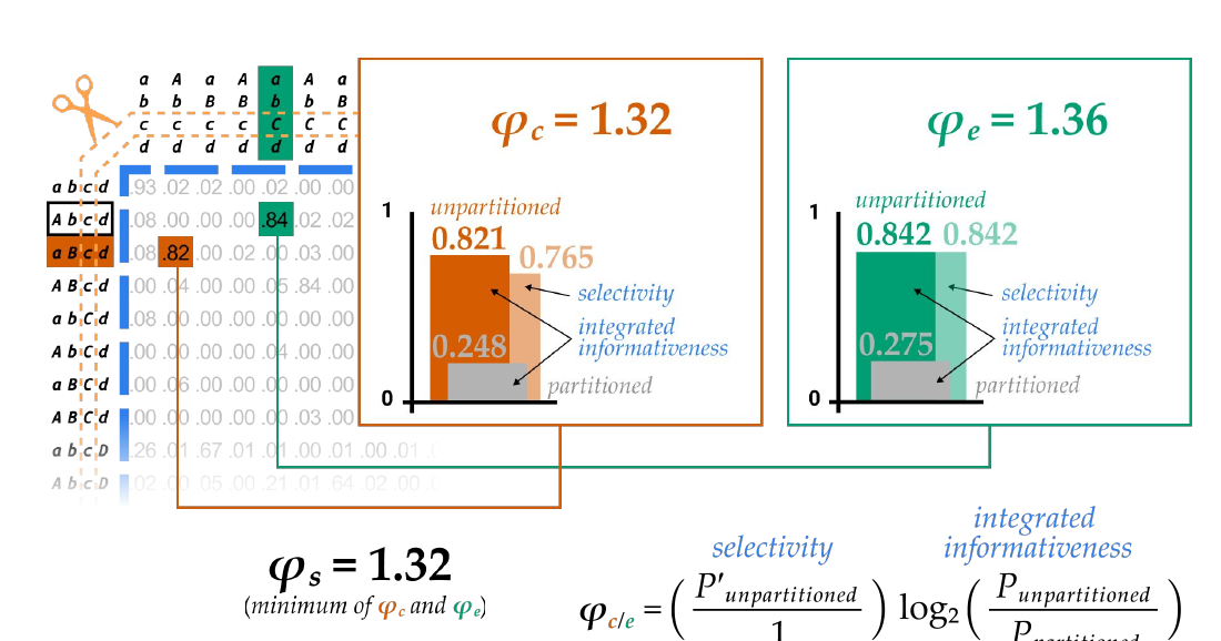
[At left is the TPM of the candidate system, with an orange pair of scissors and dashed orange lines across its column headings marking the partition, the current state *Abcd* boxed, the cause state *aBcd* marked in orange (.82) and the effect state *abCd* in green (.84). Lines lead to two bar charts on axes from 0 to 1. The orange chart, headed "φc = 1.32," has a tall orange bar labelled "unpartitioned" (0.821), a paler bar labelled "selectivity" (0.765), and a grey bar labelled "partitioned" (0.248); the gap between unpartitioned and partitioned is labelled "integrated informativeness." The green chart, headed "φe = 1.36," has an unpartitioned bar (0.842), a selectivity bar of the same height (0.842), and a partitioned bar (0.275). Below, "φs = 1.32 (minimum of φc and φe)" stands beside the formula
$$\varphi_{c/e} = \left( \frac{P'_{\text{unpartitioned}}}{1} \right) \log_2 \left( \frac{P_{\text{unpartitioned}}}{P_{\text{partitioned}}} \right)$$
with its factors labelled "selectivity" and "integrated informativeness." A red "(click)" prompt invites the reader to advance.]
### From intrinsic information to integrated information (slides 2–5)
Recall from the [information postulate](https://www.iit.wiki/axioms-and-postulates/information#h.lnlbeg807l4) that we found the specific [cause–effect state](https://www.iit.wiki/glossary#h.tp4brteczc2p) of the system in its current state.
We did this by calculating the intrinsic information (***ii***) for the cause state and effect state.
Now, applying the [integration postulate](https://www.iit.wiki/axioms-and-postulates/integration#h.1019venrnats), we aim to calculate the system's **integrated (intrinsic) information**—its **φs** value. This measures the degree to which the system in its current state specifies its cause–effect state as a *whole set of units*.
The calculation of **φs** is similar to that of ***ii***. The key difference, we will see, lies in the informativeness factor: it will become **integrated informativeness** through [partitioning](https://www.iit.wiki/glossary#h.tbsgfc5m3fti) operations.
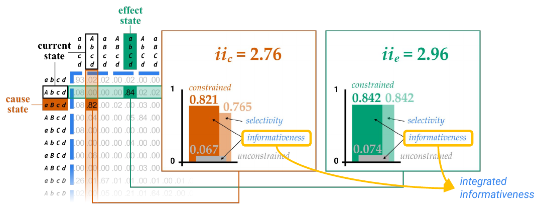
[The TPM and the two bar charts from the Information deck: *ii*c = 2.76 (constrained 0.821, selectivity 0.765, unconstrained 0.067) and *ii*e = 2.96 (constrained 0.842, selectivity 0.842, unconstrained 0.074). The label "informativeness" in each chart is boxed in yellow, and yellow arrows lead from both to the words "integrated informativeness," the factor that will replace it.]
### The partition (slides 6–10)
We start by making a **partition**, illustrated on the substrate model.
Recall that this partition includes these specific [cuts](https://www.iit.wiki/glossary#h.80uue04tp7vf) among parts ***Ab***, ***c***, and ***d***. For details, see the [integration postulate](https://www.iit.wiki/axioms-and-postulates/integration#h.1019venrnats) slides and the [FAQ: What is a valid partition?](https://www.iit.wiki/faqs/technical#h.2xou8qbtjul1)
Here, we are illustrating the [minimum partition](https://www.iit.wiki/glossary#h.uxjtor35txjh)—the one that will give us the final **φs** value of this system. But recall from the [integration postulate](https://www.iit.wiki/axioms-and-postulates/integration#h.1019venrnats) that we would have to calculate normalized **φs** for every possible partition to discover the minimum.
Like when calculating ***ii***, we will assess this partition by calculating **φ** on the cause side (φc) and effect side (φe) independently.
We will start with calculating φe, which means we treat the **current state** as our input and the **effect state** as our output.
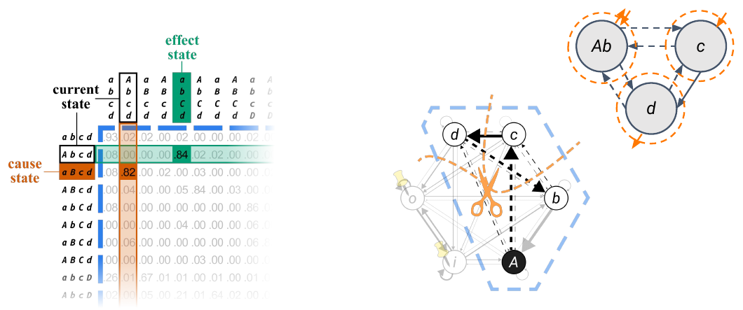
[Beside the TPM is the substrate graph of the candidate, with A ON and the other units OFF. Dashed orange lines and an orange pair of scissors divide it into the parts A and B, C, and D, and the arrows crossing between the parts are drawn dashed where they are cut; the arrow from C to D stays solid. At upper right, the same partition is drawn as a graph of three large grey circles labelled *Ab*, *c* and *d*, each ringed by a dashed orange circle marked with small orange cut marks: *Ab* on both its incoming and outgoing side, *c* on its incoming side, and *d* on its outgoing side. Dashed arrows run between *Ab* and *c* and from *d* to *Ab*; a solid arrow runs from *c* to *d*. On slide 10, the cause state is removed from the TPM, leaving the current-state row and the effect state.]
### Two TPMs for the effect side (slides 11–16)
To calculate φe, we will use two different TPMs:
- **Unpartitioned TPM** (right): this is the effect TPM for the intact substrate—the same one we used when calculating [informativeness](https://www.iit.wiki/glossary#h.a31pyyr9r104) in the previous step of [computing intrinsic information](https://www.iit.wiki/unfolding#h.z5hwahniml0v).
- **Partitioned TPM** (left): this TPM describes the transition probabilities for a counterfactual, partitioned substrate—that is, the probabilities we would expect if there were no causal interactions among the parts where the specific cuts of the partition have been made.
We will use these two TPMs to calculate the two factors needed for φe—*integrated informativeness* and *selectivity*.
But first, let's take an intermezzo:
How do we transform the intact, unpartitioned TPM into the "counterfactual," partitioned TPM?
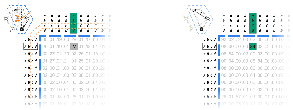
[Two 16-by-16 effect TPMs stand side by side, each with a small substrate graph above it. On the left, the partitioned TPM has dashed orange cut lines across its column headings, and a small graph with scissors. Its current-state row, *Abcd*, reads .29 .01 .19 .01 .27 .01 .18 .01 …, and the entry for the effect state *abCd*, .27, is shaded grey. On the right, the unpartitioned TPM's current-state row reads .08 .00 .00 .00 .84 .02 .02 .00 …, with the entry .84 for *abCd* shaded green. On slide 16, both TPMs appear on a grey background with a large arrow pointing from the unpartitioned TPM to the partitioned one, marked with a question mark.]
### The intact TPM as a state-by-node TPM (slides 17–20)
Let's consider the [MIP](https://www.iit.wiki/glossary#h.uxjtor35txjh) of this system again (right) and see how it alters the intact TPM.
Recall that the TPM can be equivalently shown using a [state-by-node](https://www.iit.wiki/glossary#h.clm375b2y9cx) representation, which will be more useful to explain partitioning.
As introduced in the [intrinsicality step](https://www.iit.wiki/unfolding#h.5qi5tc64lye6), the state-by-node TPM shows the probability that each unit will turn on (gray columns) given a specific input state of the system (far-left column).
Now let's see what happens to this TPM when we apply the partition step by step.
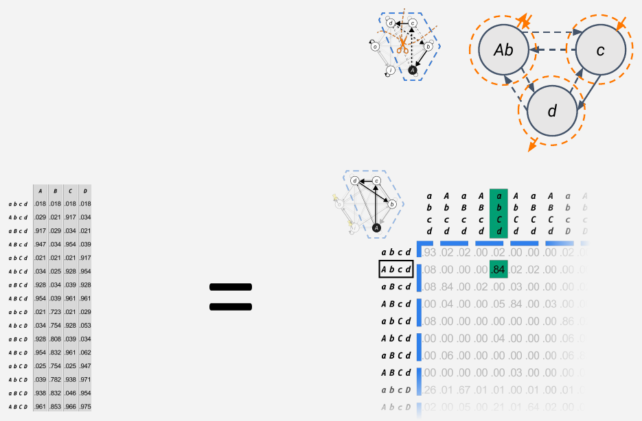
[From here to slide 65 the slides have a grey background. At upper right is the graph of the parts *Ab*, *c* and *d* with their cuts, and beside it a small substrate graph with scissors. At left is the intact state-by-node TPM of the candidate, a large equals sign, and the intact state-by-state effect TPM. The state-by-node TPM reads (each entry is the probability that the unit heading the column is ON after one update, given the input state of the row):
| input state | A | B | C | D |
|---|---|---|---|---|
| *abcd* | .018 | .018 | .018 | .018 |
| *Abcd* | .029 | .021 | .917 | .034 |
| *aBcd* | .917 | .029 | .034 | .021 |
| *ABcd* | .947 | .034 | .954 | .039 |
| *abCd* | .021 | .021 | .021 | .917 |
| *AbCd* | .034 | .025 | .928 | .954 |
| *aBCd* | .928 | .034 | .039 | .928 |
| *ABCd* | .954 | .039 | .961 | .961 |
| *abcD* | .021 | .723 | .021 | .029 |
| *AbcD* | .034 | .754 | .928 | .053 |
| *aBcD* | .928 | .808 | .039 | .034 |
| *ABcD* | .954 | .832 | .961 | .062 |
| *abCD* | .025 | .754 | .025 | .947 |
| *AbCD* | .039 | .782 | .938 | .971 |
| *aBCD* | .938 | .832 | .046 | .954 |
| *ABCD* | .961 | .853 | .966 | .975 |
These are the same numbers as in the Unfolding – Intrinsicality deck (the rows with background state *io*).]
### One TPM per part, and the cuts (slides 21–28)
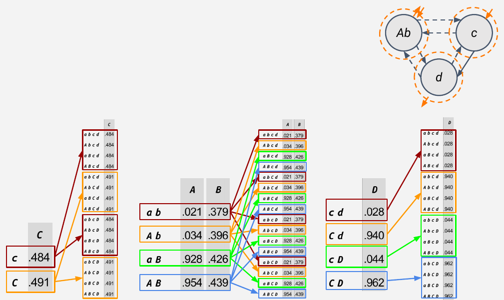
First, we separate the single state-by-node TPM into one TPM per part.
Note that each of the TPMs has every unit of the candidate complex represented on the input side.
This indicates that each part still has potential connections with every part of the system (every unit to/from every unit).
Next, we apply the cuts to each of the parts—that is, we [marginalize out](https://www.iit.wiki/glossary#h.ckhrytbflshv) all input units whose influence on the relevant part are (potentially) affected by the cut applied.
The end result will be these partitioned state-by-node TPMs for each part.
The cut to part ***Ab*** severs both incoming and outgoing connections, so the partitioned TPM only captures the causal power of ***Ab*** over itself.
The cut to part ***c*** severs all incoming connections, so the partitioned TPM only captures the [self-loop](https://www.iit.wiki/glossary#h.1yi7dnebw142) of unit C.
The cut to part ***d***, however, only severs outgoing connections, which is why the input in the partitioned TPM includes the causal power of unit C on D. (Note that units A and B are not present as inputs since the cut to part ***Ab*** severed its outgoing connections.)
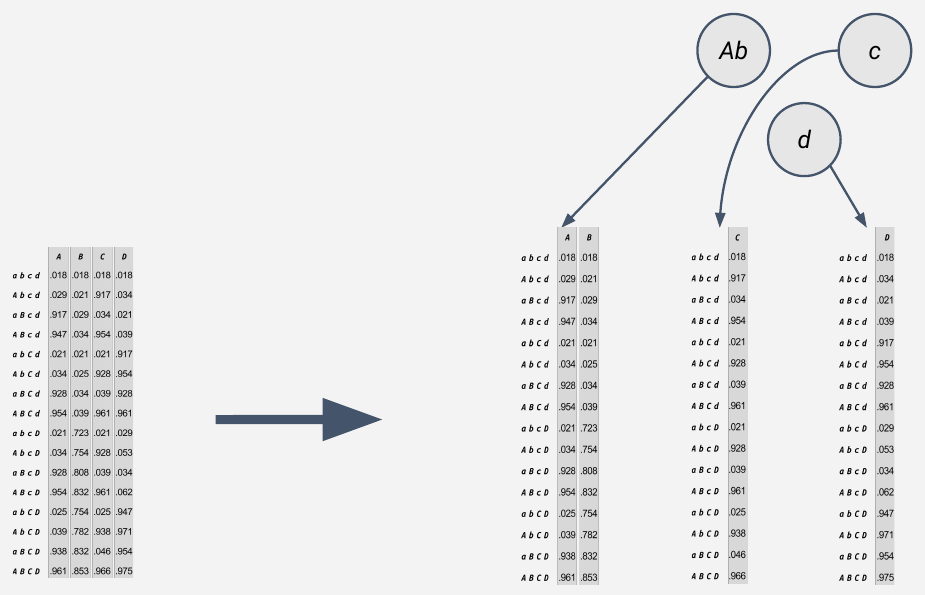
[A large arrow leads from the intact state-by-node TPM at left to three tall tables at right, one per part, each still with all 16 input states of ABCD: a table with columns A and B for part *Ab*, a table with column C for part *c*, and a table with column D for part *d*. Arrows lead from three grey circles labelled *Ab*, *c* and *d* down to their tables. On slide 23 the circles are joined by arrows in every direction, since no cut has been made yet.]
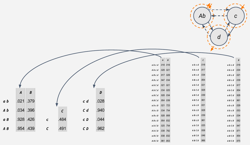
[Curved arrows lead from the three intact part TPMs at right to three small partitioned part TPMs at left, and the graph of the parts at upper right shows the cuts. The partitioned part TPMs are:
| part *Ab*: input | A | B |
|---|---|---|
| *ab* | .021 | .379 |
| *Ab* | .034 | .396 |
| *aB* | .928 | .426 |
| *AB* | .954 | .439 |
| part *c*: input | C |
|---|---|
| *c* | .484 |
| *C* | .491 |
| part *d*: input | D |
|---|---|
| *cd* | .028 |
| *Cd* | .940 |
| *cD* | .044 |
| *CD* | .962 |
The inputs of part *Ab* are A and B only, the input of part *c* is C only, and the inputs of part *d* are C and D. On slides 26–28, callout boxes point to each table with the three sentences given above.]
### Marginalizing out inputs for part c (slides 29–43)
Let's now isolate the cut to part ***c*** to see how we marginalize out units A, B, and D to get the partitioned TPM.
Note that we'll be using italics and letter case to refer to parts (since they're in a state), and roman to refer to the units generically.
We start with the intact state-by-node TPM for part ***c***.
Then we apply the cut, which in this case means we should marginalize out all inputs to ***c*** from other parts, leaving only unit C's self-loop intact.
Let's see what happens step-by-step, one input unit at a time:
We'll graphically separate units A and B temporarily since we'll have to deal with their connections to C individually.
1. Marginalize out unit A by averaging across input states where only A varies.
2. Marginalize out B in the same way from the resulting TPM, to obtain the probabilities that C turns on, independently of A and B.
3. Marginalize out D in the same way.
For these two input states, units B, C, and D are in state ***bcd***, while A is in both its available states, ***A*** and ***a***.
So, to find the probability that C turns ON for input state ***bcd*** (with A marginalized out), we take the average of the intact TPM for these two states:
(0.018 + 0.917) / 2 = 0.467
And repeat for all states of BCD
Now we have isolated part ***c*** from part ***Ab***.
But ***d*** can still have causal power over ***c***.
Now part ***c*** has been completely isolated from any outside influence; its only cause–effect power is from itself over itself.
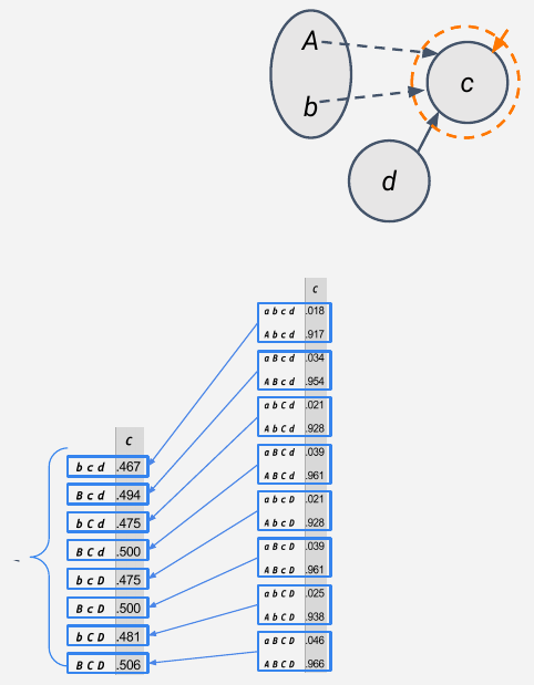
[In the graph of parts at top, part *Ab* is drawn as an elongated oval with *A* and *b* inside it, each with its own dashed arrow to *c*, whose incoming side is cut. Below, the intact column C of the state-by-node TPM is grouped by blue boxes into eight pairs of rows that differ only in the state of A (*abcd* and *Abcd*, *aBcd* and *ABcd*, and so on), and a blue line leads from each pair to its average in a new table with the eight states of BCD:
| input (A marginalized out) | C |
|---|---|
| *bcd* | .467 |
| *Bcd* | .494 |
| *bCd* | .475 |
| *BCd* | .500 |
| *bcD* | .475 |
| *BcD* | .500 |
| *bCD* | .481 |
| *BCD* | .506 |
On slides 36 and 37, the first pair is highlighted and the average .467 is worked out in a callout box.]
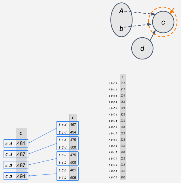
[The eight-row table is grouped into four pairs that differ only in B, and lines lead from each pair to its average in a four-row table: *cd* .481, *Cd* .487, *cD* .487, *CD* .494.]
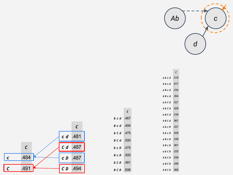
[The four-row table is grouped into two pairs that differ only in D (blue for *cd* and *cD*, red for *Cd* and *CD*), and lines lead to the final two-row table for part *c*: *c* .484, *C* .491. In the graph of parts at top, *A* and *b* are merged back into *Ab*, and only the dashed arrow from *d* to *c* is still drawn. On slide 43 a yellow check mark is placed beside the finished table, which moves to the lower left corner.]
### Marginalizing out inputs for part Ab (slides 44–48)
The same procedure can be applied to part ***Ab*** to find its partitioned TPM.
Again, all units in other parts are marginalized out of the inputs, leaving only units A and B to make a difference to their own subsequent state.
For example, to find the probability that A or B turns ON for input state ***ab*** (with units C and D marginalized out), we take the average of the intact TPM for both states of C and D:
For ***A***: (0.018 + 0.021 + 0.021 + 0.025) / 4 = 0.021
For ***B***: (0.018 + 0.021 + 0.723 + 0.754) / 4 = 0.379
Now we have the partitioned TPMs for parts ***c*** and ***Ab***.
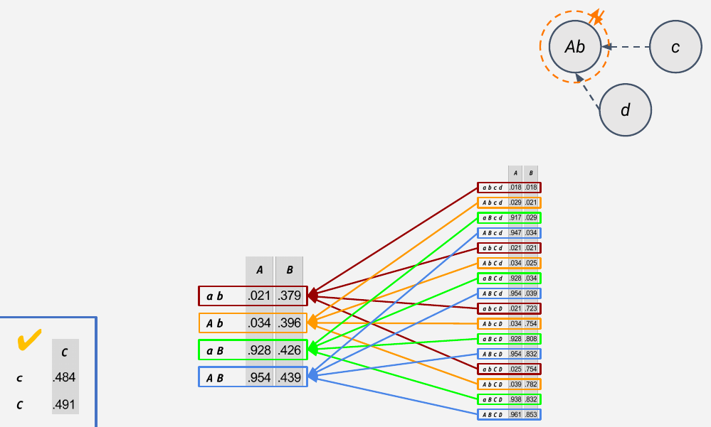
[The intact TPM of part *Ab*, columns A and B, is shown at right with its 16 rows boxed in four colours: dark red for the rows in which A and B are in state *ab*, orange for *Ab*, green for *aB* and blue for *AB*. Arrows in the same colours lead from each set of four rows to its average in the partitioned table of part *Ab* (*ab* .021 .379; *Ab* .034 .396; *aB* .928 .426; *AB* .954 .439). The finished table of part *c*, with its check mark, is at lower left. On slide 46 only the four dark red rows are drawn, with a callout box giving the calculation for *ab*.]
### Marginalizing out inputs for part d (slides 49–54)
Finally, when applying the cut to part ***d***, only the inputs from A and B are marginalized out.
Note, however, that the reason why units A and B are marginalized out is not the cut to part ***d*** (which only cuts outgoing connections). It's rather because of the outgoing cut to part ***Ab*** in the previous step.
As a rule of thumb, whenever a part has an incoming cut, we can obtain its "part TPM" without worrying about other cuts (as we did for parts ***c*** and ***Ab***). But whenever a part has a purely outgoing cut (like ***d*** in our case), we have to consider the cuts to other parts to obtain the part TPM.
Following the same procedure as before, we marginalize out units A and B from the intact TPM of part ***d*** to obtain its partitioned TPM.
As before, we average across rows of the intact TPM where the state of units C and D are identical.
Now we have the TPMs of the three parts causally separated from one another according to the partition.
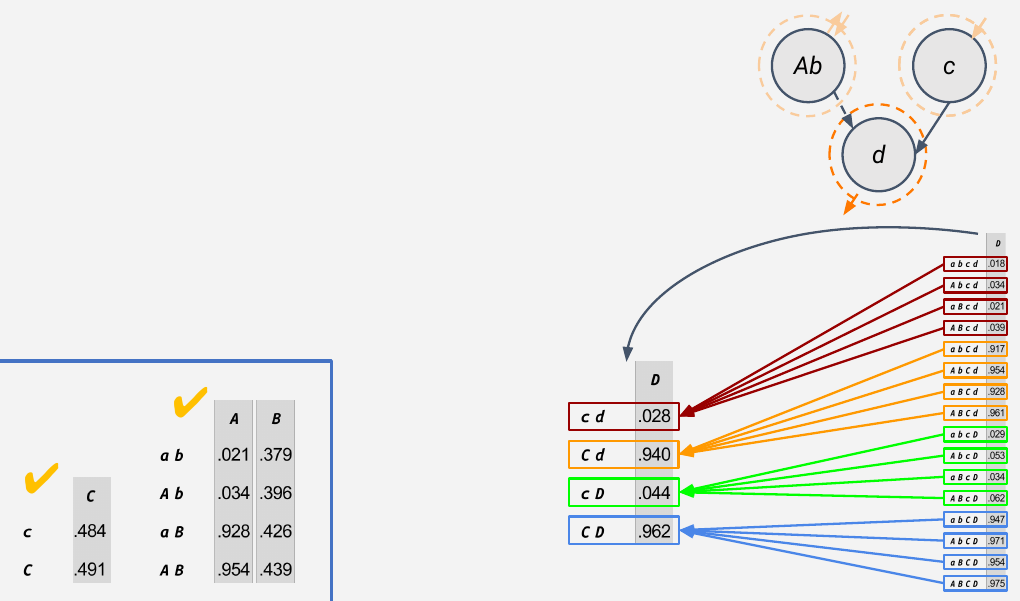
[The intact column D is shown at right with its 16 rows boxed in four colours by the state of C and D (dark red for *cd*, orange for *Cd*, green for *cD*, blue for *CD*), and arrows lead from each set of four rows to its average in the partitioned table of part *d* (*cd* .028, *Cd* .940, *cD* .044, *CD* .962). In the graph of parts at top, part *d* is highlighted with its outgoing cut, and the other two parts are faded. The finished tables of parts *c* and *Ab*, each with a check mark, are at lower left.]
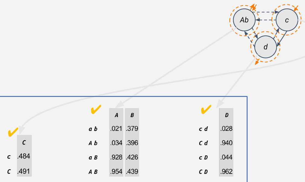
[The three partitioned part TPMs, for *c*, *Ab* and *d*, stand side by side in a blue frame, each with a yellow check mark, and faint arrows lead from the graph of parts at top to each of them.]
### Rebuilding the partitioned system TPM (slides 55–63)
The next step to obtain the partitioned system TPM is to combine the separate part TPMs appropriately. This can be thought of as rebuilding the state-by-node TPMs of the system from the part TPMs.
Let's focus on part ***c*** first. We reintroduce the units we just marginalized out, but making sure that their state makes no difference to the output state of the part (i.e., the relevant probabilities do not depend on whether the reintroduced unit is ON or OFF).
In simple terms, this means we just copy the same value in all these rows.
And here are the mappings for parts ***Ab*** and ***d***.
Next, we simply merge them together into a single state-by-node TPM.
This state-by-node TPM can now be transformed back into a state-by-state representation by simple multiplication.
For example, the probability for the system transition from ***AbcD*** to ***aBcd*** is:
P(*aBcd* | *AbcD*) = P(*a* | *AbcD*) * P(*B* | *AbcD*) * P(*c* | *AbcD*) * P(*d* | *AbcD*)
P(*aBcd* | *AbcD*) = (1 – 0.034) * 0.396 * (1 – 0.484) * (1 – 0.044)
[Each partitioned part TPM is expanded into a 16-row table, with coloured boxes and arrows showing which rows receive which value. For part *c*, the value .484 is copied into every row in which C is OFF, and .491 into every row in which C is ON. For part *Ab*, the four rows of its table are copied into the rows with the matching states of A and B. For part *d*, the four rows are copied into the rows with the matching states of C and D. On slide 57, a callout box carries the sentence about copying.]
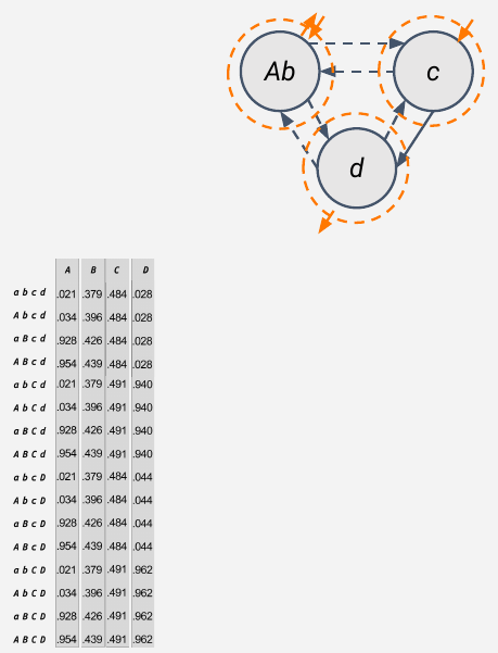
[The three expanded tables are merged into one partitioned state-by-node TPM of the whole candidate system:
| input state | A | B | C | D |
|---|---|---|---|---|
| *abcd* | .021 | .379 | .484 | .028 |
| *Abcd* | .034 | .396 | .484 | .028 |
| *aBcd* | .928 | .426 | .484 | .028 |
| *ABcd* | .954 | .439 | .484 | .028 |
| *abCd* | .021 | .379 | .491 | .940 |
| *AbCd* | .034 | .396 | .491 | .940 |
| *aBCd* | .928 | .426 | .491 | .940 |
| *ABCd* | .954 | .439 | .491 | .940 |
| *abcD* | .021 | .379 | .484 | .044 |
| *AbcD* | .034 | .396 | .484 | .044 |
| *aBcD* | .928 | .426 | .484 | .044 |
| *ABcD* | .954 | .439 | .484 | .044 |
| *abCD* | .021 | .379 | .491 | .962 |
| *AbCD* | .034 | .396 | .491 | .962 |
| *aBCD* | .928 | .426 | .491 | .962 |
| *ABCD* | .954 | .439 | .491 | .962 |
On slide 59, arrows lead from the three expanded tables into the merged one.]
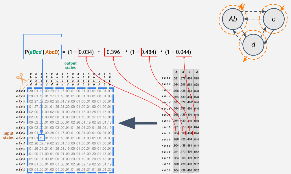
[A large arrow leads from the partitioned state-by-node TPM at right to the partitioned state-by-state TPM at left, which has scissors and dashed orange cut lines across its column headings. The row *AbcD* of the state-by-node TPM (.034 .396 .484 .044) is boxed in red, and red lines lead from each of its four values to the equation above, and from the equation to its entry in the state-by-state TPM, .19, in row *AbcD* and column *aBcd*.]
### Comparing the partitioned and intact system (slides 64–65)
In sum, the partitioned TPM provides a counterfactual version of the original system, but one in which certain parts of the substrate are causally isolated from one another.
By comparing how the intact system causally constrains itself vs. the partitioned one, we can check whether its cause–effect power is integrated (i.e., [irreducible](https://www.iit.wiki/glossary#h.sw1ddv976914)).
[The partitioned and unpartitioned effect TPMs, as in the image for slide 13, are joined by a double-headed arrow marked with a question mark.]
### Integrated informativeness and selectivity on the effect side (slides 66–74)
Now, we can finally return to how *integrated informativeness* and *selectivity* are computed. We need two probabilities:
- **Partitioned** probability: this is the probability of the current state leading to the effect state in the partitioned substrate—as simply read off of the left TPM.
- **Unpartitioned** probability: this is the probability of the same state transition in the intact substrate—as read off of the right TPM. (Note that this was called the "constrained" probability in the [information step](https://www.iit.wiki/unfolding#h.z5hwahniml0v).)
We can now calculate *integrated informativeness*, which we can crudely think of as the integrated "raw power" of the system: the smaller the partitioned probability is relative to the unpartitioned, the more integrated "raw power" the system has over itself.
Note that it's the same as the [informativeness](https://www.iit.wiki/glossary#h.a31pyyr9r104) formula, but now using unpartitioned and partitioned probabilities rather than constrained and unconstrained ones.
Like in the information step, the *selectivity* factor measures the degree to which the integrated informativeness is concentrated over the effect state.
We denote this with P' because, for the cause-side computation, it will be different from the P in the integrated informativeness factor.
$$\varphi_e = \left( \frac{P'_{\text{unpartitioned}}}{1} \right) \log_2 \left( \frac{P_{\text{unpartitioned}}}{P_{\text{partitioned}}} \right)$$
$$1.36 = \left( \frac{0.842}{1} \right) \log_2 \left( \frac{0.842}{0.275} \right)$$
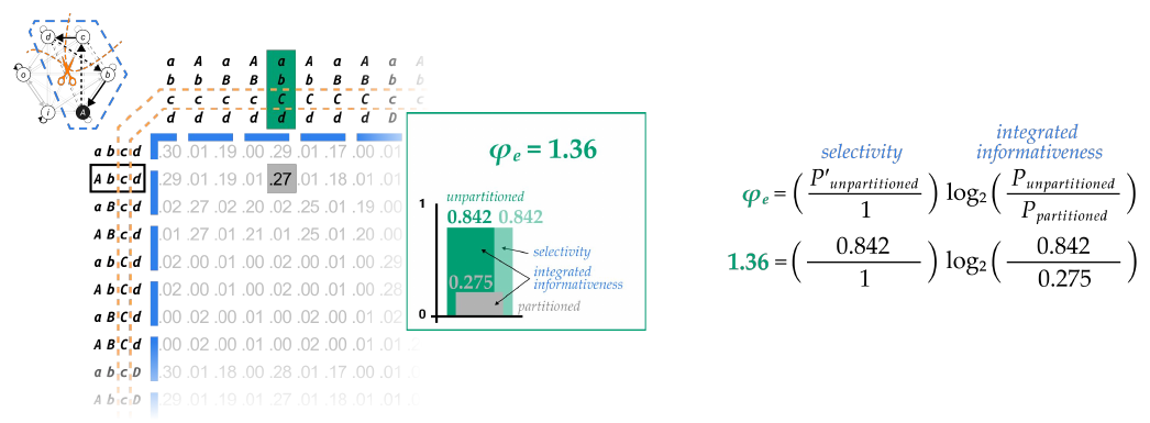
[Beside the partitioned TPM is a green bar chart headed "φe = 1.36": an unpartitioned bar (0.842), a selectivity bar of the same height (0.842), and a grey partitioned bar (0.275), with the gap between unpartitioned and partitioned labelled "integrated informativeness." To the right, the formula with its factors labelled, and below it the numbers substituted. On slide 68, a line leads from the entry .27 in the partitioned TPM to the partitioned bar; on slide 69, a line leads from .84 in the unpartitioned TPM to the unpartitioned bar; on slide 73, a callout box carries the sentence about P'.]
### The cause side (slides 75–83)
Turning now to the cause side, to calculate φc, we will treat the **cause state** as the input and the **current state** as the output.
Like for φe, we will use the partitioned TPM (left) and unpartitioned TPM (right) to calculate the informativeness factor.
But unlike before, the selectivity factor is not simply taken as the unpartitioned probability, which is why it is marked by P'.
This is because we must "take the perspective" of the current state to quantify the cause information it specifies. We can imagine this as "looking backward" from the current state to consider what the most-likely cause must have been.
Hence, we use the "backward" probability found by applying Bayes' rule to the "forward" probabilities in the cause TPM, which yields P' (see [FAQ: How do we obtain the "backward" probabilities needed for cause selectivity?](https://www.iit.wiki/faqs/technical#h.uj8qdrmujwi)).
$$\varphi_c = \left( \frac{P'_{\text{unpartitioned}}}{1} \right) \log_2 \left( \frac{P_{\text{unpartitioned}}}{P_{\text{partitioned}}} \right)$$
$$1.32 = \left( \frac{0.765}{1} \right) \log_2 \left( \frac{0.821}{0.248} \right)$$
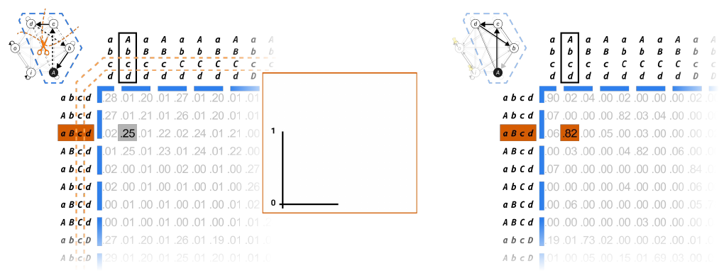
[Two cause TPMs stand side by side, each with the current state *Abcd* boxed as an output column and the cause state *aBcd* shaded orange as an input row. On the left, the partitioned cause TPM, with scissors and dashed orange cut lines, has the entry .25 for the transition from *aBcd* to *Abcd*, shaded grey. On the right, the unpartitioned cause TPM has the entry .82 for the same transition, shaded orange. An empty bar chart framed in orange stands between them.]
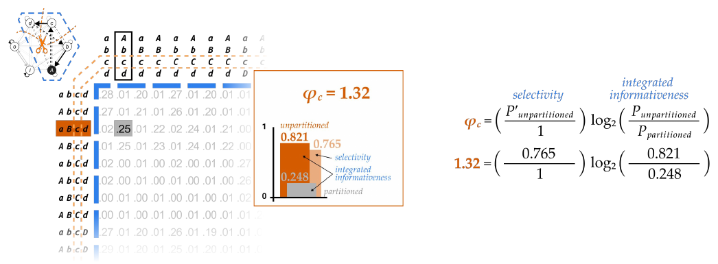
[Beside the partitioned cause TPM is an orange bar chart headed "φc = 1.32": an unpartitioned bar (0.821), a shorter selectivity bar (0.765), and a grey partitioned bar (0.248), with the gap between unpartitioned and partitioned labelled "integrated informativeness." To the right, the formula with its factors labelled, and below it the numbers substituted. On slide 77 only the partitioned bar is drawn; on slide 78 a line leads from .82 in the unpartitioned TPM to the unpartitioned bar.]
### The system integrated information (slides 84–85)
Recall from the [integration postulate](https://www.iit.wiki/axioms-and-postulates/integration#h.1019venrnats) that we take φs to be the minimum between the φc and φe for the [minimum partition](https://www.iit.wiki/glossary#h.uxjtor35txjh). Since we are depicting the minimum partition here, we can therefore conclude that φs is 1.32—the value of φc.
As a final note, if φs were 0 for the minimum partition, it would mean that candidate system ***Abcd*** is reducible. We would thus discard it as a substrate of consciousness and begin the analysis again with a new candidate—for example, subset ***bcd*** or superset ***Abcdo***.
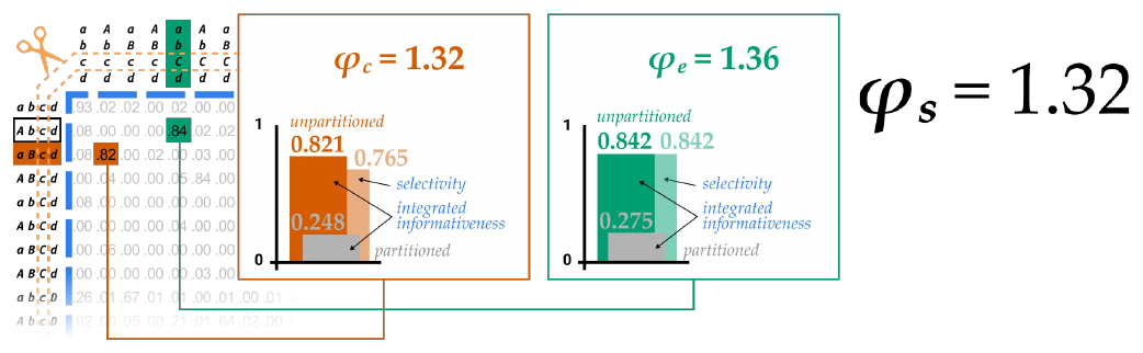
[The partitioned TPM with the cause and effect states marked, the orange bar chart for φc = 1.32 and the green bar chart for φe = 1.36, and, in large type at right, "φs = 1.32."]
### Summary slide (slide 86)
[The closing slide, labelled "summary," repeats the diagram from slide 1: the partitioned TPM, the bar charts for φc = 1.32 and φe = 1.36, "φs = 1.32 (minimum of φc and φe)," and the formula for φ.]
## Slideshow 4: Unfolding - composition - distinctions
Source page: [Computing Φ (technical)](https://www.iit.wiki/unfolding), step 6: Composition (distinctions)
Source deck: [Unfolding - composition - distinctions](https://docs.google.com/presentation/d/1siGj7WxwcRD5AhXtcGigMpobHevyLYNhMy-IPPwXcLc/edit) (100 slides)
### Title slide (slide 1)
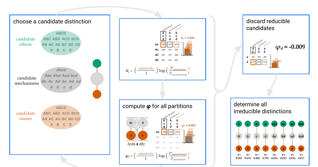
[A flow chart of five boxes linked by grey arrows. The first box, "choose a candidate distinction," shows three ovals listing the candidates: a green oval of candidate effects (the subsets of *ABCD*, in upper case), a grey oval of candidate mechanisms (the subsets of *Abcd*, in the system's current state) and an orange oval of candidate causes (the subsets of *ABCD*), beside a small distinction icon (a green effect circle above a grey mechanism circle above an orange cause circle); at its foot is the caption "repeat for all candidates on cause and effect sides." An arrow leads to "compute *ii* for all states," with the repertoire table for *bcd*–*AC* (maximum *ii*c = 1.656) and the formula for intrinsic information, and from there down to "compute φ for all partitions," with the partition *bc*/*a* × *d*/*c*, its table (φc = 0.035) and the formula for φc. A brace leads to two outcomes: "discard reducible candidates," with the table for candidate *Ab* and φd = −0.009, and "determine all irreducible distinctions," with the row of eight distinctions and their φd values shown in the image for slide 99 below. A long arrow loops back from the φ box to the first box. A red "(click)" prompt invites the reader to advance.]
### Choosing a candidate distinction (slides 2–9)
Recall that a distinction comprises three elements: a **mechanism**, **cause purview**, and **effect purview**.
Given that our system is in state ***Abcd***, we can consider any subset of the [powerset](https://www.iit.wiki/glossary#h.of3eml7gj8qf) of ***Abcd*** to be a [candidate](https://www.iit.wiki/glossary#h.8mzotxp600xu) mechanism.
Let's focus on candidate mechanism ***bcd***. We have already seen in the [composition postulate](https://www.iit.wiki/axioms-and-postulates/composition#h.uyfhol2todl) slides that it specifies a distinction with cause ***ac*** and effect ***abd***. We'll now see how we calculated that.
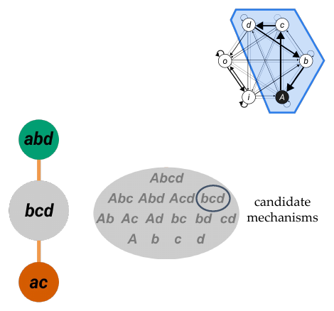
[At top right is the substrate graph of six units, with the candidate system *A*, *B*, *C*, *D* inside a blue hexagon, *A* ON (black) and the others OFF. Below it, a vertical distinction is drawn as three circles joined by orange lines: a green effect circle *abd* at the top, a grey mechanism circle *bcd* in the middle and an orange cause circle *ac* at the bottom. Beside it is a grey oval labelled "candidate mechanisms," listing the fifteen subsets of *Abcd* by size (*Abcd*; *Abc*, *Abd*, *Acd*, *bcd*; *Ab*, *Ac*, *Ad*, *bc*, *bd*, *cd*; *A*, *b*, *c*, *d*), with *bcd* circled. On slides 2 and 3 the circles are empty.]
First, we have to consider this candidate mechanism over every possible cause purview and every possible effect purview. Here we've illustrated just a few random ones.
Notice that the mechanism state is set (all OFF) because this is already "inherited" from the system state.
But these purview labels are roman uppercase to indicate that we'll have to look at every possible state of these units.
We will first calculate φc over cause purview ***AC***, and demonstrate how we discover its irreducible cause to be ***ac***.
φc means φ on the cause side, while φe means φ on the effect side. They are calculated separately, and φd ("distinction phi") is the minimum between the two.
To do this, we first need a TPM of the mechanism–purview pair–one that captures how the various states of cause purview ***AC*** transition to mechanism state ***bcd***.
Let's take a brief intermezzo to get the TPM for ***bcd***–***AC***.
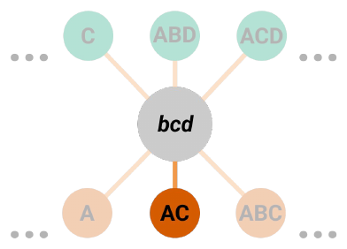
[The grey mechanism circle *bcd* sits in the middle, with faint lines to three green candidate effect purviews above (*C*, *ABD*, *ACD*) and three orange candidate cause purviews below (*A*, *AC*, *ABC*); rows of dots on either side stand for the many others. From slide 7 on, the cause purview *AC* is drawn in solid orange and its line is emphasized. This small diagram, with *AC* highlighted, stays in the top-right corner of the following slides as a reminder of which pair is being computed.]
### Intermezzo 1: The TPM for a mechanism–purview pair (slides 10–16)
We've left this little image as a reminder that we're focusing on ***bcd***–***AC***, but all of these steps have to be taken for every mechanism–purview pair on the cause side and effect side.
The TPM for the mechanism–purview pair **BCD**–**AC** can be obtained from the full [cause TPM](https://www.iit.wiki/glossary#h.8xc8ssy80ys) for system **ABCD** in four steps:
1. Obtain the [state-by-node TPM](https://www.iit.wiki/glossary#h.clm375b2y9cx) from the system TPM of **ABCD**.
2. Marginalize out any units not present on the input side of the mechanism–purview pair.
3. Ignore any units not present on the output side of the mechanism–purview pair.
4. Compute the state-by-state TPM for the mechanism–purview pair.
Let's look at each step in turn.
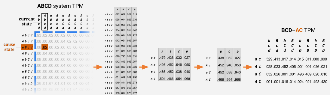
[A row of five tables linked by orange arrows. At left is the "ABCD system TPM" (the 16-by-16 cause TPM), with the current state *Abcd* boxed as an output column and the cause state *aBcd* marked in orange (.82). It becomes the 16-by-4 state-by-node TPM (step 1), then a 4-by-4 table with only *A* and *C* left as inputs (step 2), then a 4-by-3 table with only *B*, *C* and *D* left as outputs (step 3), and finally the 4-by-8 state-by-state "BCD–AC TPM" (step 4). Each table is shown in the images below, and its values are given in the tables that follow. On slide 11 only the first and last tables are shown, joined by a single arrow.]
#### Step 1: The state-by-node TPM (slides 17–18)
**1. Obtain the state-by-node TPM from the system TPM of ABCD.**
This transformation is useful for the sake of visualization (but not strictly necessary). See the [state-by-node TPM](https://www.iit.wiki/glossary#h.clm375b2y9cx) glossary entry for how it's done.
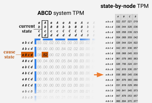
[At left is the "ABCD system TPM," a state-by-state cause TPM with input states as rows and output states as columns; the column for the current state *Abcd* is boxed and labelled "current state," and the row for *aBcd* is marked in orange and labelled "cause state," with its entry .82 highlighted. The table fades out to the right and bottom. An orange arrow leads to the "state-by-node TPM," which gives, for each of the 16 input states, the probability that each of *A*, *B*, *C* and *D* is ON:]
| Input state | A | B | C | D |
|---|---|---|---|---|
| abcd | .022 | .037 | .021 | .019 |
| Abcd | .036 | .044 | .926 | .036 |
| aBcd | .928 | .058 | .039 | .023 |
| ABcd | .954 | .068 | .959 | .042 |
| abCd | .026 | .044 | .024 | .922 |
| AbCd | .042 | .051 | .936 | .957 |
| aBCd | .938 | .068 | .045 | .933 |
| ABCd | .961 | .078 | .965 | .963 |
| abcD | .026 | .795 | .024 | .031 |
| AbcD | .042 | .819 | .936 | .057 |
| aBcD | .938 | .860 | .045 | .036 |
| ABcD | .961 | .878 | .965 | .066 |
| abCD | .031 | .819 | .029 | .950 |
| AbCD | .049 | .841 | .945 | .973 |
| aBCD | .947 | .878 | .053 | .957 |
| ABCD | .966 | .894 | .970 | .977 |
#### Step 2: Marginalizing out units on the input side (slides 19–22)
**2. Marginalize out any units not present on the input side of the mechanism–purview pair**
Since the purview is on the cause side in this mechanism–purview pair, we are interested in transition probabilities *from* the different possible purview states. Therefore, we make sure that *purview* units (**A** and **C**) are the only ones left as inputs in the resulting TPM.
For mechanism–purview pairs on the effect side, we do the same operation but only the *mechanism* units remain on the input side.
We use [unconditional marginalization](https://www.iit.wiki/glossary#h.ckhrytbflshv) as was introduced in the [integration step](https://www.iit.wiki/unfolding#h.534kz5mn6s9r) (starting around slide 29). We simply take an average over values in the rows where the relevant units are in a particular state (e.g., ***ac***).
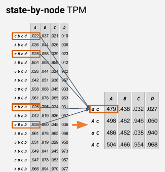
[The state-by-node TPM from slide 18, with the four rows in which *A* and *C* are both OFF (*abcd*, *aBcd*, *abcD*, *aBcD*) boxed in orange; lines lead from their *A* entries (.022, .928, .026, .938) to the entry .479 in the row *ac* of a smaller table beside it, which is also boxed. The smaller table has one row for each state of *A* and *C*:]
| Input state | A | B | C | D |
|---|---|---|---|---|
| ac | .479 | .438 | .032 | .027 |
| Ac | .498 | .452 | .946 | .050 |
| aC | .486 | .452 | .038 | .940 |
| AC | .504 | .466 | .954 | .968 |
#### Step 3: Ignoring units on the output side (slides 23–27)
**3. Ignore any units not present on the output side of the mechanism–purview pair**
Just as we removed any irrelevant units from the input side by *marginalizing*, we now remove irrelevant units from the output side by *ignoring*.
Here we ignore unit **A** since it is not part of the relevant mechanism **BCD** (the output in our current example).
And, again, if this were the effect side, the outputs would be the purview units (not mechanism units).
We can ignore the irrelevant output units, as opposed to marginalizing them out, due to the assumption of [conditional independence](https://en.wikipedia.org/wiki/Conditional_independence): the state of a given unit is independent of the state of any other unit, conditional on the past state of their inputs.
We now have the state-by-node TPM for our mechanism–purview pair.
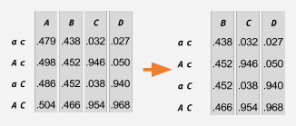
[The 4-by-4 table from step 2, and beside it, after an orange arrow, the same table with column *A* removed. On slide 27 the second table is labelled "state-by-node BCD–AC TPM":]
| Input state | B | C | D |
|---|---|---|---|
| ac | .438 | .032 | .027 |
| Ac | .452 | .946 | .050 |
| aC | .452 | .038 | .940 |
| AC | .466 | .954 | .968 |
#### Step 4: The state-by-state TPM (slides 28–30)
**4. Compute the state-by-state TPM for the mechanism–purview pair.**
As presented elsewhere (e.g., the [intrinsicality slides](https://www.iit.wiki/unfolding#h.5qi5tc64lye6), starting at 29), the state-by-state TPM can be obtained straightforwardly by multiplication (again applying the assumption of conditional independence).
For example, the purview state ***Ac*** transitions to ***BCd*** with ~40.6% probability.
$$.452 \times .946 \times (1 - .050) = 0.406$$
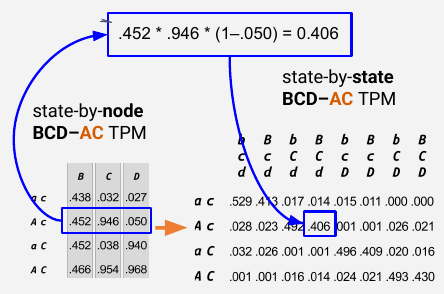
[At left is the "state-by-node BCD–AC TPM," and after an orange arrow the "state-by-state BCD–AC TPM." The row *Ac* of the state-by-node TPM (.452, .946, .050) is boxed in blue, and a blue arrow leads from it to a box with the multiplication .452 × .946 × (1 − .050) = 0.406, and from there to the entry .406 in the row *Ac* and column *BCd* of the state-by-state TPM, also boxed in blue. The state-by-state TPM gives the probability of each state of *B*, *C* and *D* (columns) for each state of *A* and *C* (rows):]
| Input state | bcd | Bcd | bCd | BCd | bcD | BcD | bCD | BCD |
|---|---|---|---|---|---|---|---|---|
| ac | .529 | .413 | .017 | .014 | .015 | .011 | .000 | .000 |
| Ac | .028 | .023 | .492 | .406 | .001 | .001 | .026 | .021 |
| aC | .032 | .026 | .001 | .001 | .496 | .409 | .020 | .016 |
| AC | .001 | .001 | .016 | .014 | .024 | .021 | .493 | .430 |
### Back to the main sequence (slides 31–32)
We can now return to the main sequence. This TPM will be used to obtain all relevant quantities for mechanism–purview pair of ***bcd***–**AC**.
Note, again, that we are referring to the **mechanism** in its specific state but to the **purview** generically: we know the state of the mechanism, but *ii* will have to be calculated for all purview states.
[These slides show the state-by-state BCD–AC TPM on its own.]
### Intrinsic information for the mechanism–purview pair (slides 33–41)
First, we compute the [intrinsic information](https://www.iit.wiki/glossary#h.vkva0021by39) (*ii*) of ***bcd***–**AC** to determine its maximal cause state. For this, we need three repertoires:
- The *constrained repertoire* for the current state is simply the relevant column of the TPM. This is all we need from this TPM, so we can discard it for now.
- The *unconstrained repertoire* can be computed by taking an average over the constrained column. The word "repertoire" is a bit misleading in this case, as the number will always be the same for all input states—it is the average over the unconstrained "repertoire". We show it multiple times here to keep the symmetry.
- The *selectivity factor* can be found by transforming the constrained repertoire using Bayes' rule to find the "backward" probabilities. (See FAQ: [How do we obtain the "backward" probabilities needed for cause selectivity?](https://www.iit.wiki/faqs/technical#h.uj8qdrmujwi)) In brief, we renormalize the values in the constrained column (so that they sum to 1).
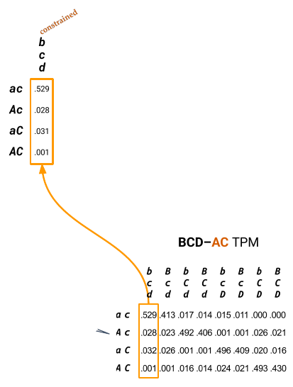
[The state-by-state BCD–AC TPM, with its first column, *bcd* (the current state of the mechanism), boxed in orange. An orange arrow leads from it up to a single column labelled "constrained," with the four values .529, .028, .031 and .001 for purview states *ac*, *Ac*, *aC* and *AC*.]
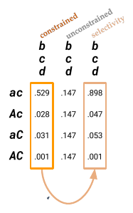
[Three columns side by side, headed "constrained," "unconstrained" and "selectivity," each labelled *bcd*. The constrained column is boxed in orange, the selectivity column is boxed in pale orange, and a curved arrow runs from the first to the third, standing for the renormalization. On slide 36 only the first two columns are shown, with an arrow from the constrained column to the unconstrained one:]
| Purview state | Constrained | Unconstrained | Selectivity |
|---|---|---|---|
| ac | .529 | .147 | .898 |
| Ac | .028 | .147 | .047 |
| aC | .031 | .147 | .053 |
| AC | .001 | .147 | .001 |
We now apply the *ii* formula for each input state:
$$ii_c = \left( \frac{\text{selectivity}}{1} \right) \log_2 \left( \frac{P_{\text{constrained}}}{P_{\text{unconstrained}}} \right)$$
$$ii_c(bcd/ac) = \left( \frac{0.898}{1} \right) \log_2 \left( \frac{0.529}{0.147} \right) = 1.656$$
$$ii_c(bcd/Ac) = \left( \frac{0.047}{1} \right) \log_2 \left( \frac{0.028}{0.147} \right) = -0.115$$
$$ii_c(bcd/aC) = \left( \frac{0.053}{1} \right) \log_2 \left( \frac{0.031}{0.147} \right) = -0.119$$
$$ii_c(bcd/AC) = \left( \frac{0.001}{1} \right) \log_2 \left( \frac{0.001}{0.147} \right) = -0.007$$
And we determine that ***ac*** is the maximal cause state of mechanism ***bcd***.
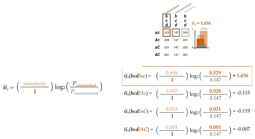
[At left is the formula for *ii*c, with "selectivity" in pale orange, "Pconstrained" in orange and "Punconstrained" in grey. At right are the four calculations above, one per purview state, with the line for *ac* (= 1.656) boxed in orange. Above them, the repertoire table is shown again with the values for *ac* boxed, beside a bar chart headed "*ii*c = 1.656": an orange constrained bar (.529), a paler selectivity bar (.898) behind it and a short grey unconstrained bar (.147).]
### φ for the mechanism–purview pair (slides 42–46)
Next, we compute the [integrated information](https://www.iit.wiki/glossary#h.o07sudcaz3vq) (φ) of ***bcd***–***ac*** over the partition illustrated here (which is the [minimal partition](https://www.iit.wiki/glossary#h.uxjtor35txjh); for more, see [FAQ: What is a valid partition?](https://www.iit.wiki/faqs/technical#h.2xou8qbtjul1)).
Note that purview ***ac*** is now also in a specific state.
To do so, we apply the integrated information formula:
$$\varphi_c = \left( \frac{\text{selectivity}}{1} \right) \log_2 \left( \frac{P_{\text{unpartitioned}}}{P_{\text{partitioned}}} \right)$$
The unpartitioned and selectivity values are the same as in the *ii* calculation (though we use the label "unpartitioned" instead of "constrained").
But we have to compute the partitioned probability. Let's take a second intermezzo to see how we obtain the "partitioned TPM" for the mechanism–purview pair over partition ***bc***/***a*** x ***d***/***c***.
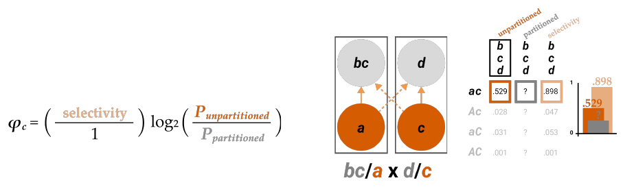
[At left is the formula for φc. In the middle, the partition is drawn as two boxes: in the first, mechanism unit *bc* (grey) sits above purview unit *a* (orange); in the second, *d* sits above *c*. Orange arrows run from each purview unit up to the mechanism units in its own box, and dotted arrows crossing between the boxes stand for the connections that are cut. The caption reads "*bc*/*a* × *d*/*c*." At right is a table with columns "unpartitioned," "partitioned" and "selectivity": for *ac* the values are .529, "?" and .898 (the other rows are faded), beside a bar chart with the unpartitioned (.529) and selectivity (.898) bars. On slide 43 only the partition is shown.]
### Intermezzo 2: The partitioned TPM for a mechanism–purview pair (slides 47–66)
Recall from the [integration step](https://www.iit.wiki/unfolding#h.534kz5mn6s9r) (starting around slide 16) that a partitioned version of a system TPM can be obtained from the intact TPM by applying these operations:
1. Obtain the [state-by-node](https://www.iit.wiki/glossary#h.clm375b2y9cx) version of the intact TPM.
2. Separate the state-by-node TPM into distinct TPMs for each part.
3. Marginalize out inputs from each "part TPM" according to the partition.
4. Recombine the part TPMs into a single "partitioned TPM" for the system.
We will follow an analogous sequence to illustrate how the partitioned probabilities are obtained for a mechanism–purview pair.
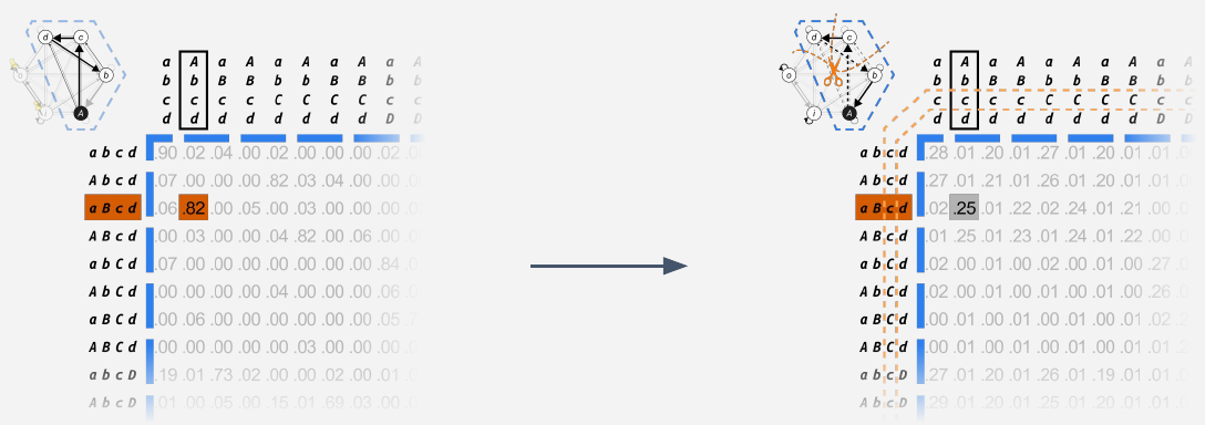
[A reminder from the integration step. At left, the candidate system's graph and its intact cause TPM, with the current state *Abcd* boxed and the cause state *aBcd* in orange (entry .82). An arrow leads to the same TPM after the system has been partitioned: the graph now shows a pair of orange scissors and dashed orange lines across some connections, and the entry for the same transition has dropped to .25.]
#### Step 1: The state-by-node version of the intact TPM (slides 51–54)
**1. Obtain the state-by-node version of the intact TPM.**
We aim to transform the state-by-state (SBS) TPM of the mechanism–purview pair **BCD**–**AC** into a [state-by-node](https://www.iit.wiki/glossary#h.clm375b2y9cx) (SBN) TPM.
Reminder: this is the TPM we obtained in **Intermezzo 1**.
Assuming all units are [conditionally independent](https://en.wikipedia.org/wiki/Conditional_independence), we find the SBN TPM by summing the relevant values in the SBS TPM.
For example, unit **C** turns on with ~94.6% probability if the input state was ***Ac***.
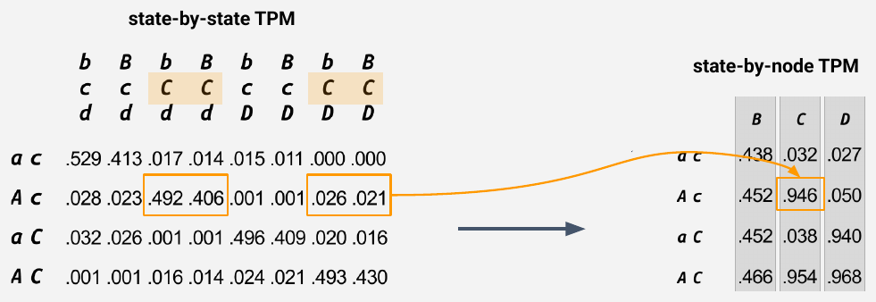
[At left is the state-by-state BCD–AC TPM from Intermezzo 1, and after an arrow the state-by-node TPM from step 3 of Intermezzo 1 (the tables above). The four columns in which *C* is ON (*bCd*, *BCd*, *bCD*, *BCD*) are shaded in their headings, and in the row *Ac* their entries (.492, .406, .026, .021) are boxed in orange; an orange line leads from them to the entry .946 (*C* given *Ac*) in the state-by-node TPM, also boxed.]
#### Step 2: Separating the TPM into part TPMs (slides 55–59)
**2. Separate the state-by-node TPM into separate TPMs for each part.**
For this next step, recall that we're working with this partition, which is the [MIP](https://www.iit.wiki/glossary#h.uxjtor35txjh).
First, we separate the columns of the intact SBN TPM, according to how the output units are partitioned.
Since we're working on the cause side, the mechanism is our output, so we separate mechanism units ***bc*** from ***d***.
Then we separate the inputs into non-overlapping sets (here, ***a*** and ***c***).
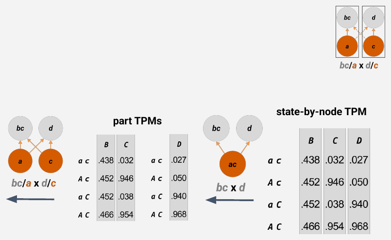
[Read from right to left. At right is the state-by-node BCD–AC TPM. An arrow leads left, under a small diagram in which the mechanism is split into *bc* and *d* over the whole purview *ac* ("*bc* × *d*"), to the "part TPMs": a table with columns *B* and *C* and a table with column *D*, each still with all four input states *ac*, *Ac*, *aC*, *AC* (the values are those of the state-by-node TPM). A second arrow leads further left, under a diagram of the partition in which *bc* receives input from *a* and *d* from *c* ("*bc*/*a* × *d*/*c*"). The partition diagram is also shown small at top right. On slides 57 and 58 only the first split (*bc* × *d*) is shown.]
#### Step 3: Marginalizing out inputs from each part TPM (slides 60–62)
**3. Marginalize out inputs from each "part TPM" according to the partition.**
We then apply the cut by marginalizing out the influence of all but one input set to each output set.
As described in the [integration slides,](https://www.iit.wiki/unfolding#h.534kz5mn6s9r) to marginalize out **C** as an input to **BC**, we take the average over its possible input states (here, ***c*** and ***C***), keeping the other input states unchanged (here, ***A***)
$$(.452 + .466)/2 = .459$$
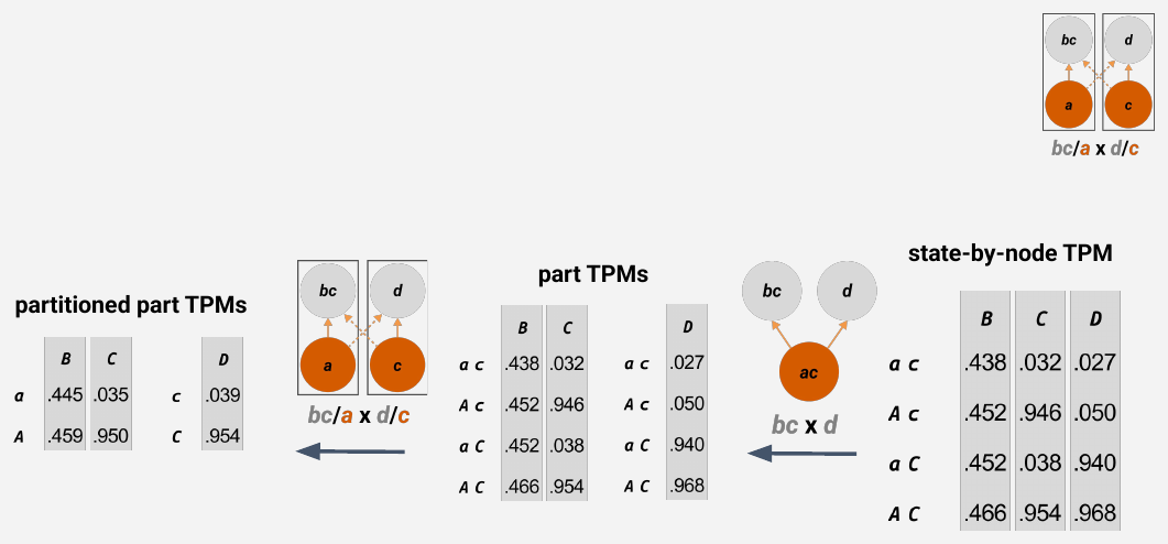
[The row of tables from slide 59, now extended at the left by the "partitioned part TPMs," which have only two input states each. On slide 62, the entries .452 (row *Ac*) and .466 (row *AC*) in the *B* column of the part TPM are boxed in red, and red arrows lead from them through a box with the average (.452 + .466)/2 = .459 to the entry .459 (*B* given *A*) in the partitioned part TPM:]
| Input | B | C |
|---|---|---|
| a | .445 | .035 |
| A | .459 | .950 |
| Input | D |
|---|---|
| c | .039 |
| C | .954 |
#### Step 4: Recombining the part TPMs (slides 63–66)
**4. Recombine the part TPMs into a single "partitioned TPM" for the system.**
We first expand the partitioned part TPMs to have the full set of input units.
For example, we simply copy these probabilities. Now, in the expanded TPM, the state of the unit added back in (here, **C**) makes no difference (is causally inert).
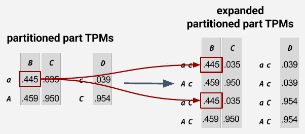
[At left are the partitioned part TPMs; after an arrow, the "expanded partitioned part TPMs," which again have a row for each of the input states *ac*, *Ac*, *aC* and *AC*. The entry .445 (*B* given *a*) is boxed in red, and red arrows copy it into the rows *ac* and *aC* of the expanded table; likewise, D's values are copied according to the state of C (.039 for *ac* and *Ac*, .954 for *aC* and *AC*). The expanded tables read as follows:]
| Input state | B | C |
|---|---|---|
| ac | .445 | .035 |
| Ac | .459 | .950 |
| aC | .445 | .035 |
| AC | .459 | .950 |
| Input state | D |
|---|---|
| ac | .039 |
| Ac | .039 |
| aC | .954 |
| AC | .954 |
And we then compute the final partitioned SBS TPM by multiplying the relevant probabilities from the SBN TPMs.
For example, these are the values we multiply to obtain the transition of ***ac*** to ***BCd***.
$$.445 \times .035 \times (1 - .039) = 0.015$$
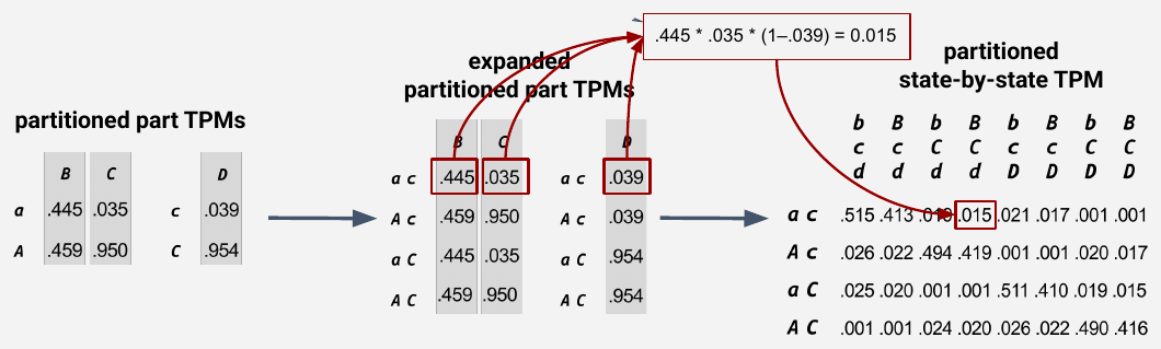
[From left to right: the partitioned part TPMs, the expanded partitioned part TPMs and the "partitioned state-by-state TPM." In the row *ac* of the expanded tables, the entries .445, .035 and .039 are boxed in red; red arrows lead from them to a box with the product .445 × .035 × (1 − .039) = 0.015, and from there to the entry .015 in the row *ac* and column *BCd* of the partitioned TPM, also boxed. The partitioned state-by-state TPM reads:]
| Input state | bcd | Bcd | bCd | BCd | bcD | BcD | bCD | BCD |
|---|---|---|---|---|---|---|---|---|
| ac | .515 | .413 | .019 | .015 | .021 | .017 | .001 | .001 |
| Ac | .026 | .022 | .494 | .419 | .001 | .001 | .020 | .017 |
| aC | .025 | .020 | .001 | .001 | .511 | .410 | .019 | .015 |
| AC | .001 | .001 | .024 | .020 | .026 | .022 | .490 | .416 |
### Computing φc for the mechanism–purview pair (slides 67–76)
We have now transformed the intact TPM into the partitioned TPM for transitions from purview **AC** to mechanism **BCD** for this specific partition (in this case the [MIP](https://www.iit.wiki/glossary#h.uxjtor35txjh)).
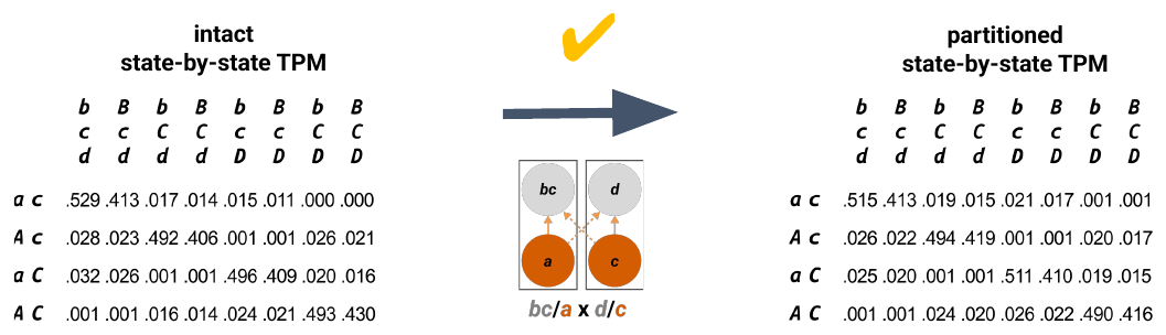
[At left is the "intact state-by-state TPM" (the BCD–AC TPM from Intermezzo 1); at right, the "partitioned state-by-state TPM" from slide 66. Between them are a large arrow, a yellow check mark and the partition diagram *bc*/*a* × *d*/*c*.]
These two TPMs give us the probabilities we need to compute the φ of ***bcd***–***ac***:
Note that we are now referring to both the **mechanism** and **purview** in their specific states because we only need to calculate φc for the maximal cause state (***ac***), which we already found.
- Recall that we already have the *unpartitioned* and *selectivity* values, obtained from the intact TPM.
- And the *partitioned* probabilities we pull from the partitioned SBS TPM.
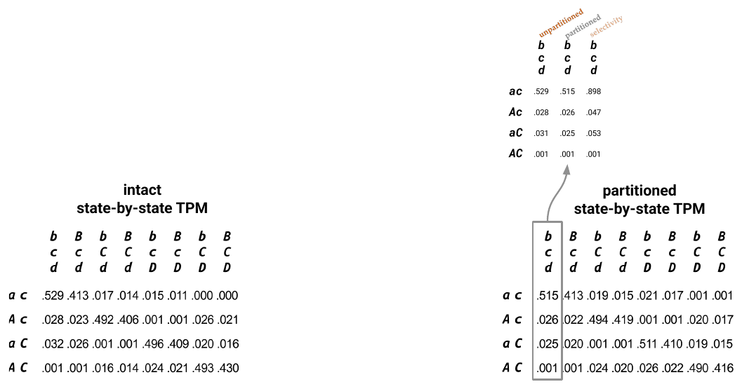
[Below, the intact and partitioned state-by-state TPMs. The *bcd* column of the partitioned TPM (.515, .026, .025, .001) is outlined in grey, and a grey arrow leads up to a table with three columns, "unpartitioned," "partitioned" and "selectivity":]
| Purview state | Unpartitioned | Partitioned | Selectivity |
|---|---|---|---|
| ac | .529 | .515 | .898 |
| Ac | .028 | .026 | .047 |
| aC | .031 | .025 | .053 |
| AC | .001 | .001 | .001 |
[On slide 69, red arrows lead instead from the *bcd* column of the intact TPM to the unpartitioned and selectivity columns.]
Now that we have our partitioned values we can compute the φc.
Recall that we can now ignore all other probabilities, since we're only interested in the state transition of ***ac*** to ***bcd***.
As mentioned already, this is indeed the MIP and thus the φc value for this mechanism–purview pair is 0.035. However, in practice, we have to check for the MIP by comparing φc of all [valid partitions](https://www.iit.wiki/faqs/technical#h.2xou8qbtjul1).
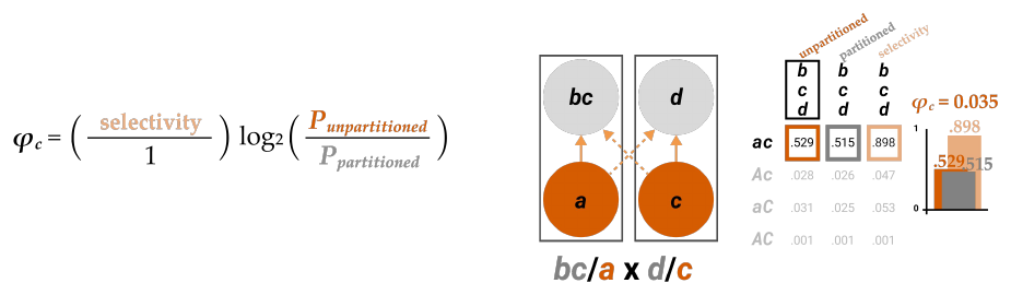
[At left, the formula for φc, with "selectivity," "Punpartitioned" and "Ppartitioned" in their colours. In the middle, the partition diagram *bc*/*a* × *d*/*c*. At right, the repertoire table with the row *ac* boxed (.529, .515, .898; the other rows faded), beside a bar chart headed "φc = 0.035": an orange unpartitioned bar (.529), a grey partitioned bar just below it (.515) and a paler selectivity bar (.898) behind them. On slide 71 the chart is not yet drawn.]
As an exercise, therefore, let's compute φc for another partition—***b***/***ac*** x ***cd***/***Ø***.
Here, φc is higher than for our MIP, as we would find for every other partition as well.
We can thus conclude that candidate cause purview ***ac*** is irreducible because its φc under the MIP is positive (φc = 0.035).
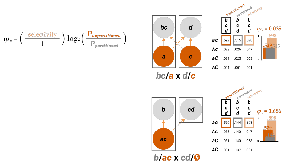
[The diagram from slide 72 is repeated at the top. Below it, the second partition is drawn: in the first box, mechanism unit *b* sits above the whole purview *ac*; in the second box, *cd* stands alone with no purview units ("*b*/*ac* × *cd*/Ø"), with a dotted arrow for the cut connection. Beside it is its repertoire table, with the row *ac* boxed, and a bar chart headed "φc = 1.686," in which the grey partitioned bar (.144) is much lower than the orange unpartitioned bar (.529):]
| Purview state | Unpartitioned | Partitioned | Selectivity |
|---|---|---|---|
| ac | .529 | .144 | .898 |
| Ac | .028 | .140 | .047 |
| aC | .031 | .140 | .053 |
| AC | .001 | .137 | .001 |
### The maximally irreducible cause (slides 77–82)
However, it is not enough to know that candidate purview ***ac*** is irreducible; the cause of ***bcd*** could be a completely different purview. Applying the [exclusion postulate](https://www.iit.wiki/glossary#h.wk5hvdb57mru), therefore, we want to find the purview that is *maximally* irreducible among all possible ones.
So let's compute φc for another candidate cause purview, **A**.
First we find its maximal state is ***a*** (with *ii* = 0.889).
Then we compute φc for ***bcd***–***a***, which is 0.017.
The φc of ***bcd***–***ac*** is higher than that of ***bcd***–***a***, and in fact of every other candidate purview. Therefore, we conclude that ***ac*** is the maximally irreducible cause of ***bcd***.
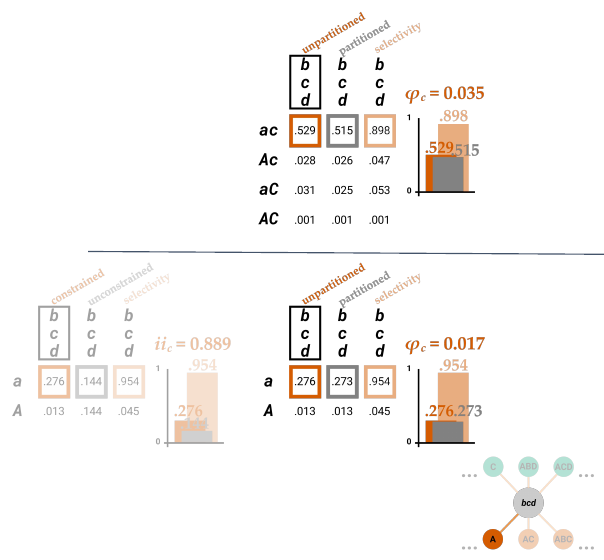
[At the top, the repertoire table and bar chart for *bcd*–*ac* (φc = 0.035) from slide 72. Below a dividing line are two tables for purview *A*, and a small reminder diagram shows *bcd* with cause purview *A* highlighted. The first, faded, table has columns "constrained," "unconstrained" and "selectivity," with the row *a* boxed and a bar chart headed "*ii*c = 0.889." The second has columns "unpartitioned," "partitioned" and "selectivity," with the row *a* boxed and a bar chart headed "φc = 0.017":]
| Purview state | Constrained | Unconstrained | Selectivity |
|---|---|---|---|
| a | .276 | .144 | .954 |
| A | .013 | .144 | .045 |
| Purview state | Unpartitioned | Partitioned | Selectivity |
|---|---|---|---|
| a | .276 | .273 | .954 |
| A | .013 | .013 | .045 |
[On slide 82 the table for *bcd*–*ac* is framed in orange, marking *ac* as the maximally irreducible cause, and the tables for *A* are faded.]
### Repeating all steps on the effect side (slides 83–87)
To fully compute distinction ***bcd***, we now have to do the same on the effect side.
The procedure on the effect side is identical to the cause side, except that the selectivity factor in *ii*e is simpler to compute: it is always identical to the constrained probability.
***bcd***'s maximally irreducible effect is over ***abd***, with φe = 0.017.
Since both ***bcd***'s cause and effect are irreducible, mechanism ***bcd*** is irreducible, and its φd = 0.017 (the [minimum](https://www.iit.wiki/glossary#h.dtwzpm4kzynp) between its φc and φe).
We now have a bona fide distinction: ***ac***–***bcd***–***abd***.
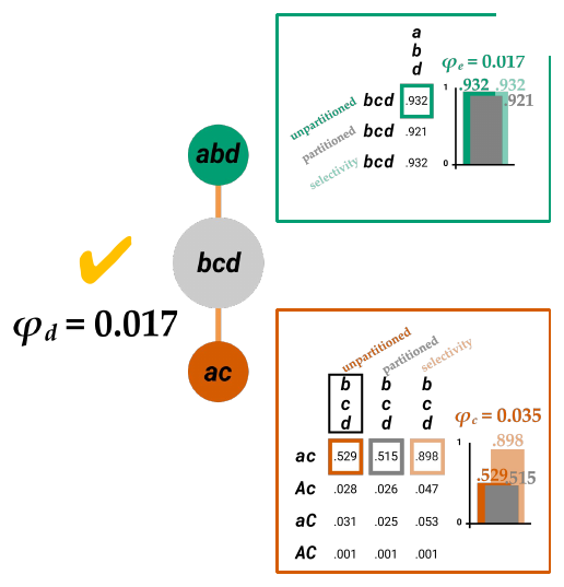
[The distinction is drawn vertically: the green effect circle *abd* at the top, the grey mechanism *bcd* in the middle and the orange cause circle *ac* at the bottom. Beside it, framed in green, is the effect-side table for *bcd* over effect purview *abd*, with rows "unpartitioned" (.932, boxed), "partitioned" (.921) and "selectivity" (.932), and a bar chart headed "φe = 0.017." Framed in orange below is the cause-side table for *bcd*–*ac* with its chart, φc = 0.035. To the left, a yellow check mark and "φd = 0.017." On slide 83 the mechanism is shown with a few candidate effect purviews (*C*, *ABD*, *ACD*) and only the cause-side table; on slides 84 and 85 the effect-side table is added.]
### Calculating φd for each candidate distinction (slides 88–93)
We then have to repeat the procedure for all candidate mechanisms: each must be tested not only with each candidate purview but also in each possible purview state.
Note again that the candidate mechanisms inherit the system state…
…but the candidate purviews are depicted without a state since we have to check every state permutation.
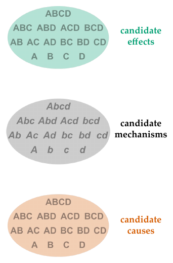
[Three ovals, one above the other. The green oval, "candidate effects," and the orange oval, "candidate causes," each list the fifteen subsets of *ABCD* in upper case, by size (*ABCD*; *ABC*, *ABD*, *ACD*, *BCD*; *AB*, *AC*, *AD*, *BC*, *BD*, *CD*; *A*, *B*, *C*, *D*). The grey oval between them, "candidate mechanisms," lists the fifteen subsets of *Abcd* in the system's current state. On slide 90 callout boxes point to the mechanism oval and the cause oval.]
The number of candidates we must assess in a system of *n* units is given by this formula:
$$\#\text{ candidates} = 2 \ast (2^N - 1) \sum_{M=1}^{N} \frac{2^M \ast N!}{M!\,(N-M)!}$$
The contents of this formula are as follows:
- *M* is the size of a candidate purview (to be iterated over)
- *N* is number of units in the system
- (*N* choose *M*) = *N*!/(*N*–*M*)!*M*! is the number of possible purview of size *M*
- 2^*M* number of purview states
- 2^*N*–1 is the number of candidate mechanisms
- 2 is needed to count cause and effect states independently
So for a four-unit system, there are 2400 candidate mechanism–purview pairs we must assess (thankfully, PyPhi does it for us).
Usually, the vast majority of these will be reducible, and thus discarded.
### A reducible candidate: Ab (slides 94–97)
For example, let's see what happens when we assess candidate mechanism ***Ab***—depicted here over a few randomly selected cause and effect purviews.
It may look promising when we calculate intrinsic information and find that (on the cause side) it is positive and maximal over ***A***.
However, when we calculate φc, we find it to be negative (–0.009).
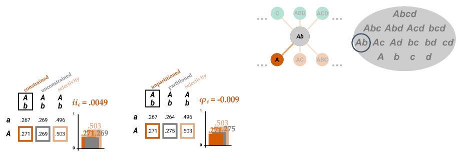
[At top, the mechanism *Ab* is drawn in grey with a few candidate effect purviews (*C*, *ABD*, *ACD*) and cause purviews (*A*, *AC*, *ABC*), with cause purview *A* in solid orange; beside it, the oval of candidate mechanisms with *Ab* circled. Below are two tables for purview *A*. The first, with columns "constrained," "unconstrained" and "selectivity," has the row *A* boxed and a bar chart headed "*ii*c = .0049." The second, with columns "unpartitioned," "partitioned" and "selectivity," has the row *A* boxed and a bar chart headed "φc = -0.009," in which the grey partitioned bar is slightly higher than the orange unpartitioned bar:]
| Purview state | Constrained | Unconstrained | Selectivity |
|---|---|---|---|
| a | .267 | .269 | .496 |
| A | .271 | .269 | .503 |
| Purview state | Unpartitioned | Partitioned | Selectivity |
|---|---|---|---|
| a | .267 | .264 | .496 |
| A | .271 | .275 | .503 |
And if we were to repeat this for every candidate cause purview, we would find this φc value to be the maximal of all candidates.
If the maximal φ of a candidate is 0 or negative, this means it is reducible. We can thus discard candidate ***Ab*** from the *Φ*-structure.
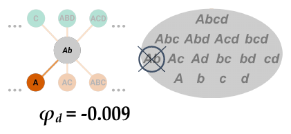
[The mechanism *Ab* with its candidate purviews, as on slide 96, and the oval of candidate mechanisms, in which *Ab* is now crossed out. Below, "φd = -0.009."]
### The irreducible distinctions (slides 98–99)
By assessing every candidate distinction in this way—on both the cause and effect sides—we find which candidates are irreducible.
There are 8 in our case, each with an associated φd value.
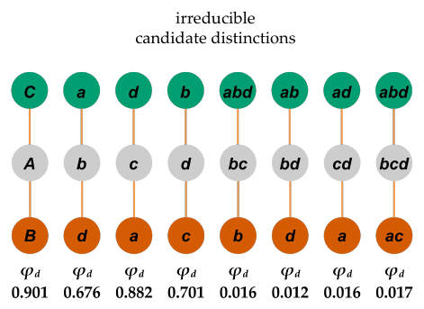
[Under the heading "irreducible candidate distinctions," eight distinctions are drawn side by side, each as a green effect circle above a grey mechanism circle above an orange cause circle, joined by orange lines, with its φd value below. On slide 98 the values are not yet shown:]
| Mechanism | Cause | Effect | φd |
|---|---|---|---|
| A | B | C | 0.901 |
| b | d | a | 0.676 |
| c | a | d | 0.882 |
| d | c | b | 0.701 |
| bc | b | abd | 0.016 |
| bd | d | ab | 0.012 |
| cd | a | ad | 0.016 |
| bcd | ac | abd | 0.017 |
### Summary (slide 100)
[The closing slide, labelled "summary," repeats the flow chart from slide 1: choose a candidate distinction, compute *ii* for all states, compute φ for all partitions, then discard reducible candidates and determine all irreducible distinctions, repeating for all candidates on cause and effect sides.]
## Slideshow 5: Unfolding - composition - relations
Source page: [Computing Φ (technical)](https://www.iit.wiki/unfolding), step 6: Composition (relations)
Source deck: [Unfolding - composition - relations](https://docs.google.com/presentation/d/18lR9iBd56UnXpJSVDBmsyk8czhS5nyIFQG0F9N-gYOM/edit) (18 slides)
### Title slide (slide 1)
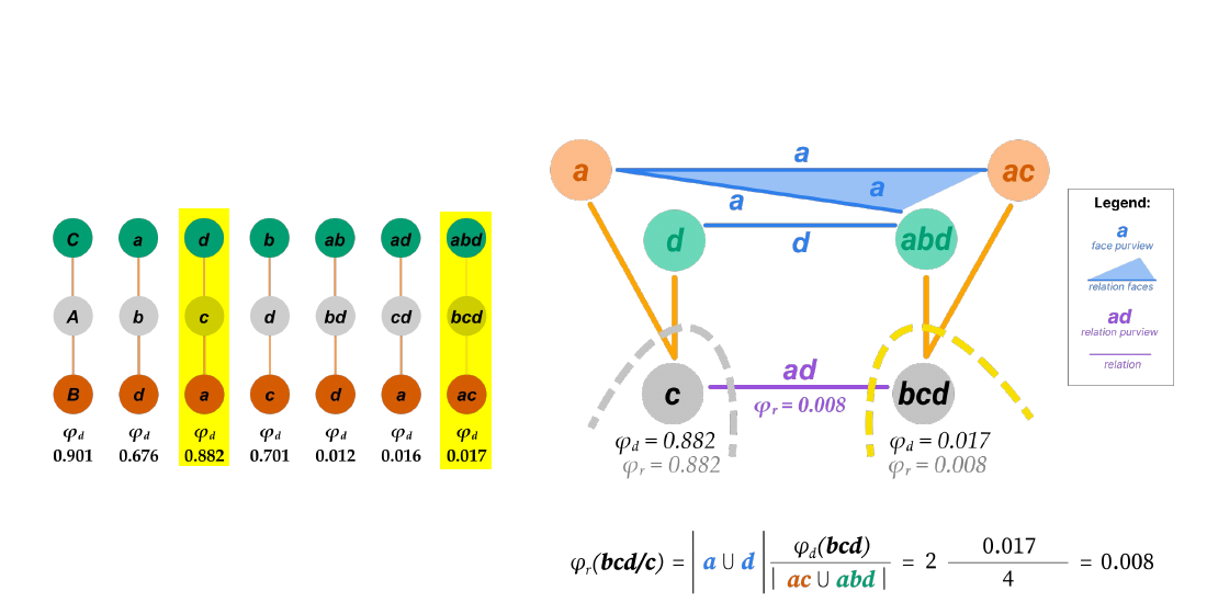
[At left is the row of the system's seven distinctions (listed in the table under slides 3–7 below), each drawn as a green effect circle above a grey mechanism circle above an orange cause circle, with its φd value beneath; the distinctions *c* and *bcd* are highlighted in yellow. In the middle, the relation between them is drawn on its own: the mechanisms *c* (φd = 0.882) and *bcd* (φd = 0.017) sit at the bottom, joined by a purple line labelled "*ad*" (the relation purview) and "φr = 0.008." Orange lines rise from each mechanism to its cause purview (*a* for *c*, *ac* for *bcd*, in orange) and green lines to its effect purview (*d* for *c*, *abd* for *bcd*, in green). Blue lines labelled *a* join *a* to *ac* and *a* to *abd*, a blue line labelled *d* joins *d* to *abd*, and a blue triangle labelled *a* joins *a*, *ac* and *abd*: these are the relation's faces. A dashed grey arc around *c* is labelled "φr = 0.882" and a dashed yellow arc around *bcd* is labelled "φr = 0.008," standing for the two ways of unbinding the relation. A legend explains the symbols: a blue letter is a face purview, a blue triangle a relation face, a purple label a relation purview, and a purple line a relation. Below is the calculation φr(*bcd*/*c*) = |*a* ∪ *d*| · φd(*bcd*) / |*ac* ∪ *abd*| = 2 × 0.017/4 = 0.008. A red "(click)" prompt invites the reader to advance.]
### The distinctions and their overlaps (slides 2–7)
At this point, we have all irreducible, congruent distinctions, with their respective φd values, but they are still unstructured.
| Mechanism | Cause | Effect | φd |
|---|---|---|---|
| A | B | C | 0.901 |
| b | d | a | 0.676 |
| c | a | d | 0.882 |
| d | c | b | 0.701 |
| bd | d | ab | 0.012 |
| cd | a | ad | 0.016 |
| bcd | ac | abd | 0.017 |
To see how they compose a specific *Φ*-structure, our next step is to determine their relations—all the ways in which the distinctions overlap over their purviews.
Let's focus on a 2nd-degree relation between distinctions ***c*** and ***bcd***, which was described in the [composition postulate](https://www.iit.wiki/axioms-and-postulates/composition#h.uyfhol2todl) (slides 35–40).
Here we've isolated the two distinctions and their relation for more precise illustration.
This is a 2nd-[degree](https://www.iit.wiki/glossary#h.xdmiiu46u8m6) relation (because it involves two distinctions, purple), which is composed by 2nd- and 3rd-degree [faces](https://www.iit.wiki/glossary#h.jbpcsbi2vw6e) (i.e., overlaps between purviews, blue).
This relation comprises two 2nd-degree faces (blue edges) with face purviews over ***a***, one 2nd-degree face with a face purview over ***d***, and one 3rd-degree face (blue area) with a face purview over ***a***.
These distinctions are related because they overlap over purview units ***a*** and ***d***.
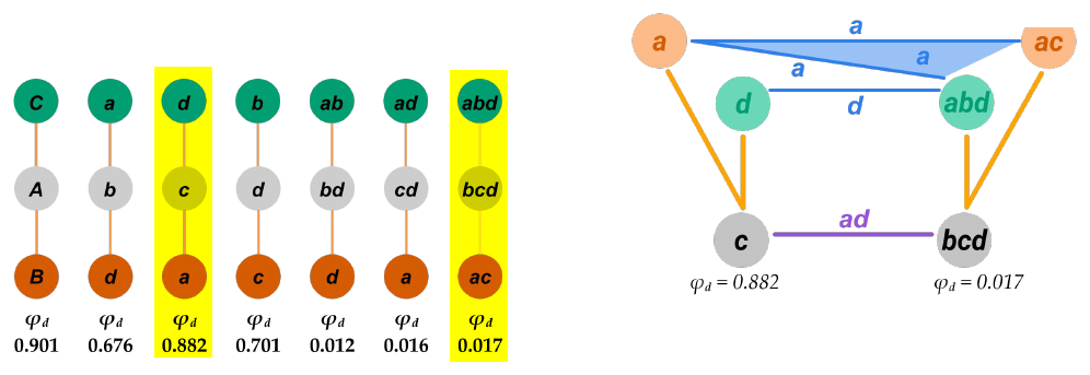
[At left, the row of seven distinctions with *c* and *bcd* highlighted in yellow. At right, the relation between *c* (φd = 0.882) and *bcd* (φd = 0.017) as described for slide 1, without the arcs and φr values: the purple line labelled *ad* joins the two mechanisms, and the blue lines and triangle mark the four faces (*a*–*ac* and *a*–*abd* over *a*, *d*–*abd* over *d*, and the triangle *a*–*ac*–*abd* over *a*). On slides 3 and 4 only the row of distinctions is shown, without highlights; on slide 7 two callout boxes carry the sentences about the faces and about the overlap over *a* and *d*.]
### Unbinding the distinctions (slides 8–11)
To assess the irreducibility of the relation, we partition or "unbind" the distinctions that constitute it, one at a time, and identify which distinction contributes *least* to the overlap (the relation MIP).
This is what is expressed in the the relations formula of [IIT 4.0](https://journals.plos.org/ploscompbiol/article?id=10.1371/journal.pcbi.1011465#sec044). Here, we will offer a simplified version focused on the relation between ***bcd*** and ***c***.
$$\varphi_r(\mathbf{d}) = \min_{d \in \mathbf{d}} \left| \bigcup_{f \in \mathbf{f}(\mathbf{d})} o^*_f \right| \frac{\varphi_d}{\left| z^*_c(d) \cup z^*_e(d) \right|}$$
Let's first calculate the φr from unbinding distinction ***bcd***.
Why one at a time? Given the current formalism in IIT 4.0, unbinding more than one distinction will always result in a higher φr than unbinding a single one.
[On slides 8–11 the relation between *c* and *bcd* is shown on its own. From slide 10 on, a dashed grey arc is drawn around *bcd*, with a faint "φr = 0.008" beneath it.]
### φr from unbinding bcd (slides 12–14)
We multiply the average φd per distinct purview unit by the size of the overlap across all faces, as shown in the formula.
$$\varphi_r(bcd/c) = \left| a \cup d \right| \frac{\varphi_d(bcd)}{\left| ac \cup abd \right|} = 2 \, \frac{0.017}{4} = 0.008$$
This means we're unbinding ***bcd*** from its relation with ***c***. |*a* ∪ *d*| is the size of the relation overlap (i.e., the union of the face overlaps); φd(*bcd*) is the φd of the distinction we're unbinding (***bcd***); and |*ac* ∪ *abd*| is the size of the union of purview units of the distinction we're unbinding (***bcd***).
- ***bcd***'s φd is .017 and its purviews contain four unique units (***a*** is repeated), so the average φd per purview unit is 0.017/4 = 0.004.
- Since the relation in question has an overlap over two units (face purviews ***a*** and ***d***), φr = 0.004*2 = 0.008.
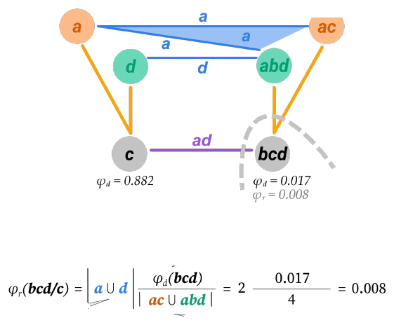
[The relation between *c* and *bcd*, with a dashed grey arc around *bcd* and "φr = 0.008" beneath it. Below is the formula, with |*a* ∪ *d*| in blue, φd(*bcd*) and |*ac* ∪ *abd*| (with *ac* in orange and *abd* in green), followed by "= 2 × 0.017/4 = 0.008." On slide 13 four callout boxes point to the parts of the formula, carrying the explanations given above.]
### φr from unbinding c, and the relation MIP (slides 15–16)
If instead we unbind distinction ***c***, we get a φr of 0.882.
$$\varphi_r(c/bcd) = \left| a \cup d \right| \frac{\varphi_d(c)}{\left| a \cup d \right|} = 2 \, \frac{0.882}{2} = 0.882$$
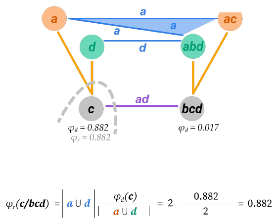
[The relation between *c* and *bcd*, now with the dashed grey arc around *c* and "φr = 0.882" beneath it. Below is the formula for φr(*c*/*bcd*), in which the denominator |*a* ∪ *d*| has *a* in orange (the cause purview of *c*) and *d* in green (its effect purview).]
Since the φr of unbinding ***bcd*** is less than that of unbinding ***c***, by the [principle of minimal existence](https://www.iit.wiki/glossary#h.dtwzpm4kzynp), we conclude that the MIP of the relation is ***bcd***/***c*** and its φr is 0.008.
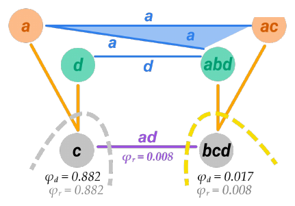
[The relation between *c* and *bcd*. The dashed arc around *c* is grey (φr = 0.882), while the dashed arc around *bcd* is now yellow (φr = 0.008), marking it as the relation MIP. The purple relation line carries "φr = 0.008" under its label *ad*.]
### All relations (slide 17)
By computing all relations in this way for all 7 distinctions, we discover 31 relations in total, with a cumulative φr of 0.932.
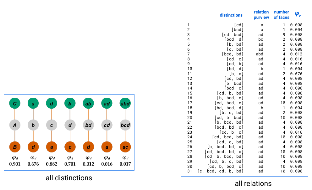
[At left, framed in blue and captioned "all distinctions," the row of seven distinctions with their φd values. At right, framed in blue and captioned "all relations," a table listing every relation with the distinctions it binds (named by their mechanisms), its relation purview, its number of faces and its φr:]
| # | Distinctions | Relation purview | Number of faces | φr |
|---|---|---|---|---|
| 1 | cd | a | 1 | 0.008 |
| 2 | bcd | a | 1 | 0.004 |
| 3 | cd, bcd | ad | 9 | 0.008 |
| 4 | bcd, d | bc | 2 | 0.008 |
| 5 | b, bd | ad | 2 | 0.008 |
| 6 | c, bd | ad | 2 | 0.008 |
| 7 | bcd, bd | abd | 4 | 0.012 |
| 8 | cd, c | ad | 4 | 0.016 |
| 9 | cd, b | ad | 4 | 0.016 |
| 10 | bd, d | b | 1 | 0.004 |
| 11 | b, c | ad | 2 | 0.676 |
| 12 | cd, bd | ad | 4 | 0.008 |
| 13 | b, bcd | ad | 4 | 0.008 |
| 14 | bcd, c | ad | 4 | 0.008 |
| 15 | cd, b, bd | ad | 4 | 0.008 |
| 16 | b, bcd, c | ad | 4 | 0.008 |
| 17 | cd, bcd, c | ad | 10 | 0.008 |
| 18 | bd, bcd, d | b | 1 | 0.004 |
| 19 | b, c, bd | ad | 2 | 0.008 |
| 20 | cd, b, bcd | ad | 10 | 0.008 |
| 21 | b, bcd, bd | ad | 4 | 0.008 |
| 22 | bcd, bd, c | ad | 4 | 0.008 |
| 23 | cd, b, c | ad | 4 | 0.016 |
| 24 | cd, bcd, bd | ad | 10 | 0.008 |
| 25 | cd, c, bd | ad | 4 | 0.008 |
| 26 | b, bcd, bd, c | ad | 4 | 0.008 |
| 27 | cd, bcd, bd, c | ad | 10 | 0.008 |
| 28 | cd, b, bcd, bd | ad | 10 | 0.008 |
| 29 | cd, b, c, bd | ad | 4 | 0.008 |
| 30 | cd, b, bcd, c | ad | 10 | 0.008 |
| 31 | c, bcd, cd, b, bd | ad | 10 | 0.008 |
[Relations 1 and 2 are self-relations, in which a single distinction's cause and effect overlap (over *a*). The relation between *c* and *bcd* worked through above is number 14. Distinction *A* takes part in no relation.]
### Summary (slide 18)
[The closing slide, labelled "summary," repeats the figure from slide 1: the row of distinctions with *c* and *bcd* highlighted, their relation with the two unbindings (φr = 0.882 and 0.008), the legend, and the calculation φr(*bcd*/*c*) = 0.008.]