# Slides: Information
*The lab's transcriptions of the decks embedded on https://www.iit.wiki/axioms-and-postulates/information: each slide's text as the deck shows it, and in square brackets a description of each diagram, which is the transcriber's and not the deck's.*
## Slideshow 1: Information Postulate - 08/2023
Source page: [Information](https://www.iit.wiki/axioms-and-postulates/information)
Source deck: [Information Postulate](https://docs.google.com/presentation/d/1wFkS7P2_EXCCPGSE18Veei1RS_AqoN33ptJ_on3ZPqw/edit) (32 slides)
### Title slide (slide 1)
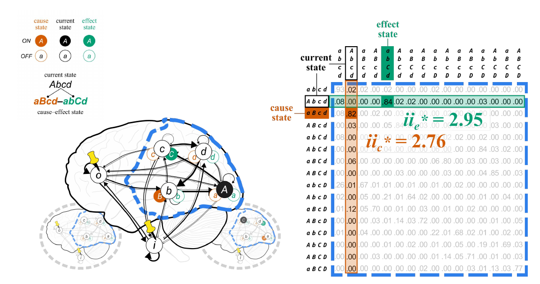
[At top left, a legend gives the colour code used throughout: a unit's cause state is shown in orange, its current state in black and its effect state in green, each as a filled circle with an uppercase letter when ON and an open circle with a lowercase letter when OFF. Beneath it, "current state *Abcd*" leads to "*aBcd*–*abCd*, cause–effect state," with the cause state in orange and the effect state in green. Below is the brain with the six units: a dashed blue line encloses the candidate system A, B, C and D, units O and I carry yellow pushpins, and each candidate unit shows its current state with small orange and green circles beside it for its cause and effect states. Two smaller, faded brains in dashed grey circles sit at the lower left and right, standing for other possible states. On the right is the TPM of the candidate system, with the current-state column (*Abcd*) boxed in black, the cause-state row (*aBcd*) marked in orange, and the effect-state column (*abCd*) marked in green. Large lettering over the table reads *ii*e* = 2.95 in green and *ii*c* = 2.76 in orange. A red "(click)" prompt invites the reader to advance.]
### From axiom to postulate (slides 2–5)
**Axiom:** Experience is *specific*: it is *this one*.
How can we formulate this [phenomenal](https://www.iit.wiki/glossary#h.8j4o0g5ssetv) property in physical terms—that is, in terms of [cause–effect power](https://www.iit.wiki/glossary#h.vlk7u52cim8x)?
**Postulate:** The cause–effect power of the substrate of consciousness must be *specific*: it must be in *this state* and select *this cause–effect state*.
Note that these slides give a conceptual overview of the postulate without going into the mathematics. Use the links to learn more about key concepts, and visit the [Computing Φ](https://www.iit.wiki/unfolding) page for technical details.
[Beneath the axiom are three overlapping round photographs (the same ones shown with slide 31 below). In front is the wiki's sample experience, a first-person view of lying on a bed with a book in a bright room with wide windows; behind it, in circles with dashed grey borders, are a building's façade with a tall window at left and a beach with waves at right, standing for other possible experiences. A blue arrow leads from the axiom to the postulate, which is set above the question.]
### The candidate system and its effect TPM (slides 6–8)
Recall that the [intrinsicality postulate](https://www.iit.wiki/axioms-and-postulates/intrinsicality#h.ffm1nm3ehxmu) guided us in isolating our [candidate substrate](https://www.iit.wiki/glossary#h.8mzotxp600xu) (**ABCD**), and "[pinning](https://www.iit.wiki/glossary#h.vq8lj719uzmz)" [background conditions](https://www.iit.wiki/glossary#h.ot008m3n2clu) (**I** and **O**).
This let us focus on only **ABCD** as both input and output, and discard units **I** and **O** from our TPM.
Note that these probabilities are only the effect TPM, which we will use throughout this deck for simplicity.
In practice, however, we work with a cause TPM and effect TPM to analyse cause power and effect power, respectively.
Technical details are in [Computing Φ: Step 3—Information](https://www.iit.wiki/unfolding#h.z5hwahniml0v).
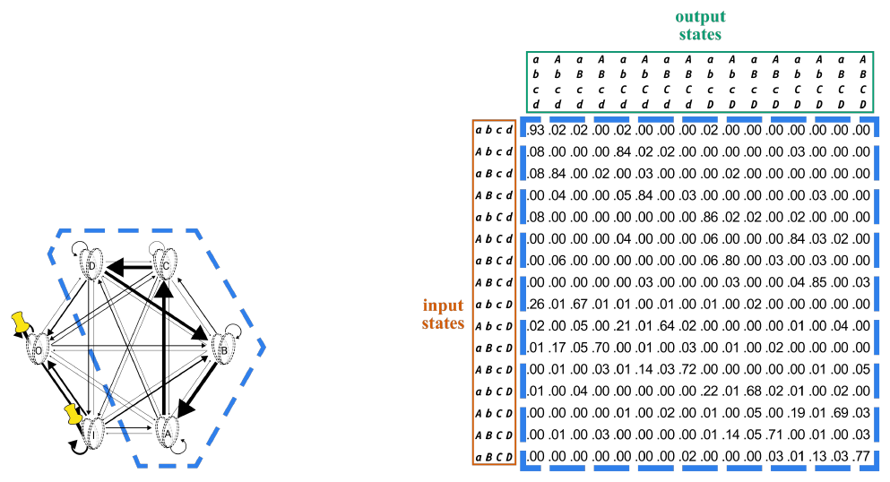
[On the left is the six-unit substrate graph, with a dashed blue hexagon around A, B, C and D and yellow pushpins on O and I. On the right is the TPM of the candidate system alone: 16 input states of ABCD down the side (from abcd to ABCD, marked "input states") and the same 16 output states across the top (marked "output states"), each entry a transition probability. The whole table is enclosed in a dashed blue box. On slide 6 the larger substrate TPM, with I and O pinned, stood in its place; on slide 8 a callout box over the table carries the note given above.]
### A specific current state (slides 9–11)
Now, the **information** postulate requires that the cause–effect power of the substrate be *specific*.
First, this means that we consider the substrate [units](https://www.iit.wiki/glossary#h.y4l991ydyf0n) to be in a specific current state—here, ***Abcd***, where lowercase italics indicates OFF and uppercase italics ON.
And on the [TPM](https://www.iit.wiki/glossary#h.rgqyfluj1zit), we are now interested in the specific row and column that correspond to this current state.
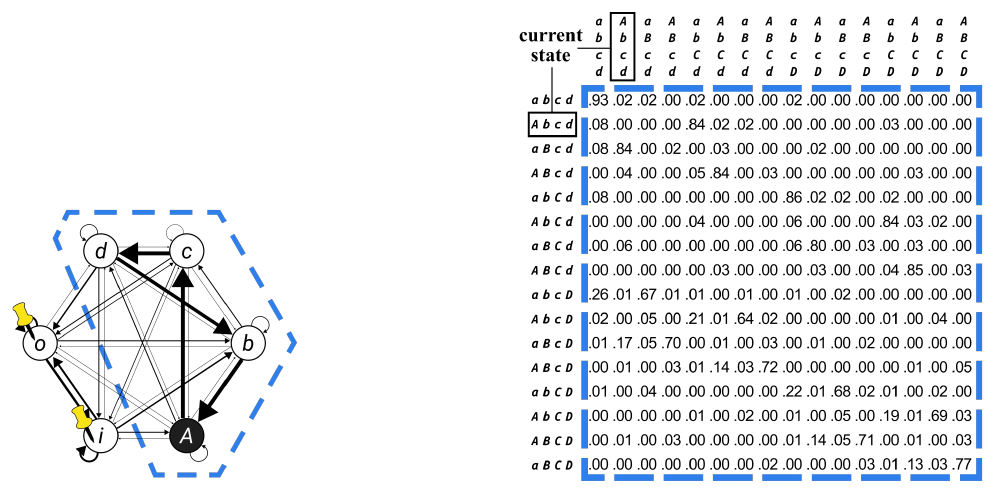
[On the substrate graph, unit A is now a filled black circle labelled *A* (ON), and B, C and D are open circles labelled *b*, *c* and *d* (OFF). In the TPM, the row for input state *Abcd* and the column for output state *Abcd* are each boxed in black, and the column is labelled "current state."]
### One cause and one effect (slides 12–13)
In one sense, the substrate is specific simply by virtue of being in its current state. But the specificity of experience must be accounted for not by the substrate *per se* but by its cause–effect power.
Hence, for its cause–effect power to be specific, the system must specify only one cause and one effect among all possible ones.
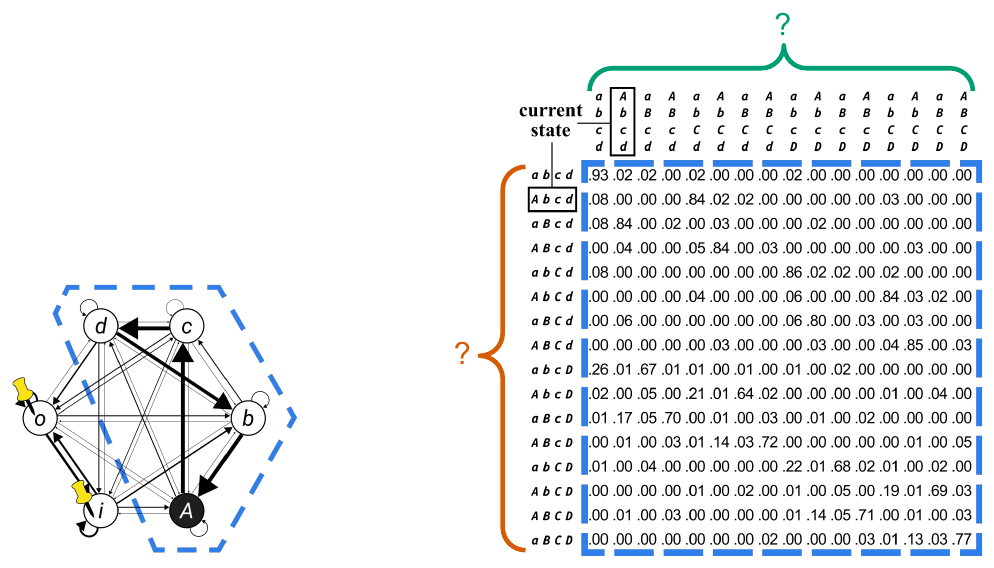
[The graph and TPM are as on slide 11. A large orange brace with a question mark spans all the rows of the TPM, standing for the possible cause states, and a large green brace with a question mark spans all the columns across the top, standing for the possible effect states.]
### The cause–effect state (slides 14–16)
In this sample system, the cause state is ***aBcd***, shown on the substrate graph and TPM.
And the effect state is ***abCd***, also shown on the substrate graph and TPM.
Together, these form the *cause–effect state* of the system.
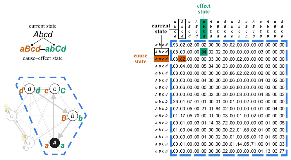
[Beside each candidate unit on the graph, its cause state is written in orange to its left and its effect state in green to its right: *d* and *d* for D, *c* and *C* for C, *B* and *b* for B, *a* and *a* for A. The background units and most arrows are faded. Above the graph, "current state *Abcd*" leads to "*aBcd*–*abCd*, cause–effect state." In the TPM, the row for input state *aBcd* is marked in orange and labelled "cause state," and its entry in the current-state column, .82, is highlighted in orange; the column for output state *abCd* is marked in green and labelled "effect state," and its entry in the current-state row, .84, is highlighted in green.]
### Not simply the highest probability (slides 17–18)
To convey the basic idea, we have depicted the cause–effect state of this system without explaining how we got it.
It may be tempting to think it is found by simply looking to the TPM squares with the highest probability (as in this example, with 0.82 and 0.84). But it is not that simple, and in some cases, the cause or effect state will not correspond to the highest transition probability.
### Intrinsic information (slides 19–21)
The cause and effect states rather aim to capture the system's "best bet" about its cause ("from which it came") and effect ("to which it's going")—*from its intrinsic perspective*.
We determine the cause–effect state by calculating the [intrinsic information](https://www.iit.wiki/glossary#h.vkva0021by39) (*ii*) of every possible cause state (highlighted column)…and every possible effect state (highlighted row) of the system in its current state.
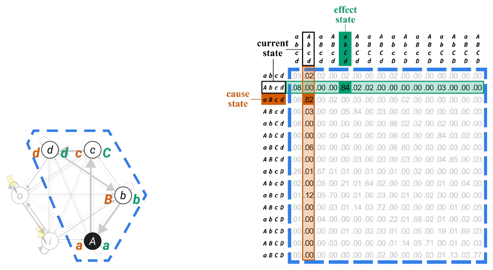
[In the TPM, the whole current-state column is shaded orange, since its entries give the probability of the current state from each possible cause state, and the whole current-state row is shaded green, since its entries give the probability of each possible effect state from the current state; all other entries are faded. In the text, "(highlighted column)" is printed in orange and "(highlighted row)" in green.]
### Maximal intrinsic information (slides 22–23)
By the [principle of maximal existence](https://www.iit.wiki/glossary#h.qof4052teerl), we choose the cause state and effect state that maximize intrinsic information (*ii*)—in this case, *ii*c = 2.76 and *ii*e = 2.95.
The details for calculating *ii* can be [found here](https://www.iit.wiki/unfolding#h.z5hwahniml0v).
The asterisk indicates the maximum.
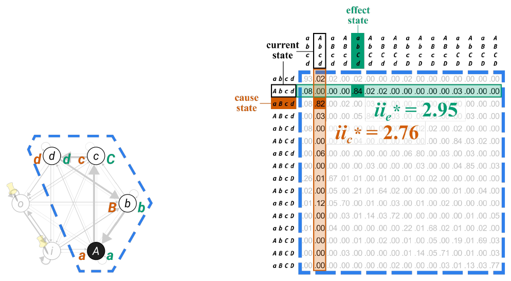
[Over the highlighted column and row of the TPM, large lettering reads *ii*e* = 2.95 in green and *ii*c* = 2.76 in orange. On slides 22 and 23, a callout box points to the asterisk with the sentence given above.]
### The charioteer analogy (slides 24–29)
Without getting into the math, the cause state or effect state that specifies maximal *ii* can be thought of as the one that strikes the optimal balance between "raw power" and "control" (called [informativeness](https://www.iit.wiki/glossary#h.a31pyyr9r104) and [selectivity](https://www.iit.wiki/glossary#h.a4n8qbkkpgw), respectively).
As a simple analogy, imagine a charioteer shafted to a single, well-trained horse. The reins are taut, and the driver has full control over the horse.
If the rider were offered a second horse—equally well-trained—he would gladly take it. This would double his "horsepower" without sacrificing control.
But if the rider were then offered a third, wild horse, who responds very little to the reins, should he take it?
Certainly not. We might expect to get one more horsepower, but from the rider's perspective, the increase in horsepower is not worth the sacrifice of control.
He would prefer the two-horse set-up, since it is the one that optimizes power and control.
[Click here](https://www.iit.wiki/unfolding#h.z5hwahniml0v) for a deeper look at how intrinsic information is conceptualized and calculated.
Image sources: [chariot](https://www.flaticon.com/free-icon/chariot_1597787), [running horse](https://www.flaticon.com/free-icon/horse-running-silhouette_35983), [bucking horse](https://www.flaticon.com/free-icon/horse-standing-on-two-back-paws-black-side-view-silhouette_35918)
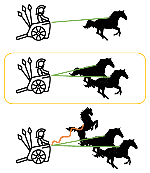
[Three black silhouettes of a charioteer in a chariot are stacked one above another. In the first, a single running horse pulls the chariot on a taut green rein. In the second, two running horses pull on taut green reins. In the third, the same two horses are joined by a bucking horse rearing on its hind legs, whose rein is orange and slack. The added pictures appear one at a time over slides 25–28; on slide 29 a rounded yellow box outlines the two-horse set-up as the preferred one.]
### Specificity implies differentiation (slides 30–31)
As a final point, recall from the information axiom that specificity implies *differentiation*: by virtue of being specific, my experience differs from a repertoire of other possible experiences, each of which is also specific, as illustrated in the figure.
Similarly, by virtue of having this specific cause–effect state (***aBcd***–***abCd***), the substrate of consciousness is differentiated from a repertoire of possible cause–effect states. This is illustrated by the smaller brains here, each of which has a different substrate state and a different cause–effect state.
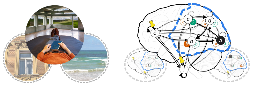
[On the left are the three overlapping round photographs: in front, the first-person view of lying on a bed with a book; behind it, in dashed grey circles, a building's façade and a beach, standing for other possible experiences. On the right is the brain with the candidate system enclosed in dashed blue, O and I pinned, and each unit shown in its current state with its cause and effect states beside it in orange and green. Below it, at left and right, are two smaller, faded brains in dashed grey circles, each with the units in a different state, standing for the repertoire of other possible cause–effect states.]
### Summary slide (slide 32)
[The closing slide, labelled "summary," pairs the axiom and postulate from slide 5 with the three photographs and the diagram from slide 1: the colour legend, "current state *Abcd*" leading to the cause–effect state *aBcd*–*abCd*, the brain with its smaller alternatives, and the TPM with *ii*e* = 2.95 and *ii*c* = 2.76.]